Quantile Regression for Counts — rq.counts • Qtools

This function is used to fit a (log-linear) quantile regression model when the response is a count variable.

Usage

rq.counts(formula, data = sys.frame(sys.parent()), tau = 0.5, subset, weights,
  na.action, contrasts = NULL, offset = NULL, method = "fn", M = 50,
  zeta = 1e-5, B = 0.999, cn = NULL, alpha = 0.05)

Arguments

formula: an object of class formula: a symbolic description of the model to be fitted.
data: an optional data frame, list or environment (or object coercible by as.data.frame to a data frame) containing the variables in the model. If not found in data, the variables are taken from environment(formula), typically the environment from which rq.counts is called.
tau: quantile to be estimated.
subset: an optional vector specifying a subset of observations to be used in the fitting process.
weights: an optional vector of weights to be used in the fitting process.
na.action: a function which indicates what should happen when the data contain NAs.
contrasts: an optional list. See the contrasts.arg of model.matrix.default.
offset: an optional offset to be included in the model frame.
method: estimation method for the fitting process. See rq.
M: number of dithered samples.
zeta: small constant (see References).
B: right boundary for uniform random noise U[0,B] to be added to the response variable (see References).
cn: small constant to be passed to Fn (see Theorem 3, Machado and Santos Silva).
alpha: significance level.

Details

A linear quantile regression model is fitted to the log–transformed response. The notation used here follows closely that of Machado and Santos Silva (2005). This function is based on routines from package quantreg (Koenker, 2016). See also lqm.counts from package lqmm (Geraci, 2014) for Laplace gradient estimation.

As of version 1.4, the transformation of the response cannot be changed. This option may be reinstated in future versions.

Value

a list of class rq.counts containing the following components

call: the matched call.
method: the fitting algorithm for rq.
x: the model matrix.
y: the model response.
tau: the order of the estimated quantile(s).
tsf: tranformation used (see also attributes(tsf)).
coefficients: regression quantile (on the log–scale).
fitted.values: fitted values (on the response scale).
tTable: coefficients, standard errors, etc.
offset: offset.
M: specified number of dithered samples for standard error estimation.
Mn: actual number of dithered samples used for standard error estimation that gave an invertible D matrix (Machado and Santos Silva, 2005).
InitialPar: starting values for coefficients.
terms: the terms object used.
term.labels: names of coefficients.
rdf: the number of residual degrees of freedom.

References

Geraci M. Linear quantile mixed models: The lqmm package for Laplace quantile regression. Journal of Statistical Software. 2014;57(13):1-29.

Geraci M and Jones MC. Improved transformation-based quantile regression. Canadian Journal of Statistics 2015;43(1):118-132.

Koenker R. quantreg: Quantile Regression. 2016. R package version 5.29.

Machado JAF, Santos Silva JMC. Quantiles for counts. Journal of the American Statistical Association. 2005;100(472):1226-37.

Author

Marco Geraci

Examples


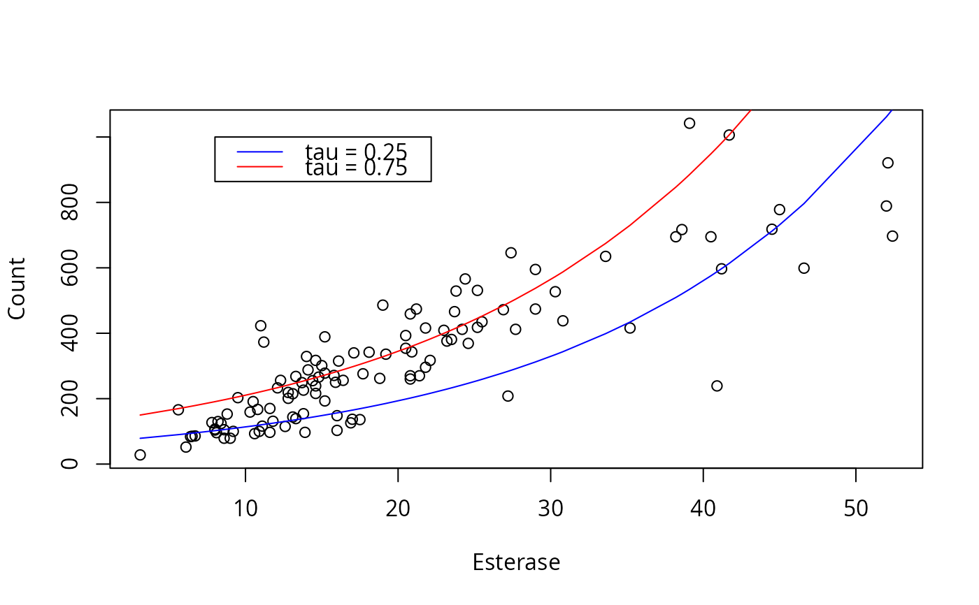
# Esterase data
data(esterase)

# Fit quantiles 0.25 and 0.75
fit1 <- rq.counts(Count ~ Esterase, tau = 0.25, data = esterase, M = 50)
coef(fit1)
#> (Intercept)    Esterase 
#>  4.19876563  0.05324203 
fit2 <- rq.counts(Count ~ Esterase, tau = 0.75, data = esterase, M = 50)
coef(fit2)
#> (Intercept)    Esterase 
#>  4.85193762  0.04943663 

# Plot
with(esterase, plot(Count ~ Esterase))
lines(esterase$Esterase, fit1$fitted.values, col = "blue")
lines(esterase$Esterase, fit2$fitted.values, col = "red")
legend(8, 1000, lty = c(1,1), col = c("blue", "red"), legend = c("tau = 0.25","tau = 0.75"))