Quantile Regression Transformation Models

These functions are used to fit quantile regression transformation models.

Usage

tsrq(formula, data = sys.frame(sys.parent()), tsf = "mcjI", symm = TRUE,
  dbounded = FALSE, lambda = NULL, conditional = FALSE, tau = 0.5,
  subset,  weights, na.action,  contrasts = NULL, method = "fn")
tsrq2(formula, data = sys.frame(sys.parent()), dbounded = FALSE, lambda = NULL,
  delta = NULL, conditional = FALSE, tau = 0.5, subset, weights, na.action,
  contrasts = NULL, method = "fn")
rcrq(formula, data = sys.frame(sys.parent()), tsf = "mcjI", symm = TRUE,
  dbounded = FALSE, lambda = NULL, tau = 0.5, subset, weights, na.action,
  contrasts = NULL, method = "fn")
nlrq1(formula, data = sys.frame(sys.parent()), tsf = "mcjI", symm = TRUE,
  dbounded = FALSE, start = NULL, tau = 0.5,
  subset,  weights, na.action, contrasts = NULL, control = list())
nlrq2(formula, data = sys.frame(sys.parent()), dbounded = FALSE,
  start = NULL, tau = 0.5, subset, weights, na.action, contrasts = NULL)

Arguments

formula: an object of class "formula" (or one that can be coerced to that class): a symbolic description of the model to be fitted. The details of model specification are given under `Details'.
data: an optional data frame, list or environment (or object coercible by as.data.frame to a data frame) containing the variables in the model. By default the variables are taken from the environment from which the call is made.
tsf: transformation to be used. Possible options are mcjI for Proposal I transformation models (default), bc for Box-Cox and ao for Aranda-Ordaz transformation models.
symm: logical flag. If TRUE (default) a symmetric transformation is used.
dbounded: logical flag. If TRUE the response is assumed to be doubly bounded on [a,b]. If FALSE (default) the response is assumed to be singly bounded (ie, strictly positive).
lambda, delta: values of transformation parameters for grid search.
conditional: logical flag. If TRUE, the transformation parameter is assumed to be known and this must be provided via the arguments lambda, delta in vectors of the same length as tau.
start: vector of length 1 + p (nlrq1) or 2 + p (nlrq2) of initial values for the parameters to be optimized over. The first one (nlrq1) or two (nlrq2) values for the transformation parameter lambda, or lambda and delta, while the last p values are for the regression coefficients. These initial values are passed to nl.fit.rqt or to optim.
control: list of control parameters of the fitting process (nlrq1). See nlControl.
tau: the quantile(s) to be estimated. See rq.
subset: an optional vector specifying a subset of observations to be used in the fitting process.
weights: an optional vector of weights to be used in the fitting process. Should be NULL or a numeric vector.
na.action: a function which indicates what should happen when the data contain NAs.
contrasts: an optional list. See the contrasts.arg of model.matrix.default.
method: fitting algorithm for rq (default is Frisch-Newton interior point method "fn").

Details

These functions implement quantile regression transformation models as discussed by Geraci and Jones (see references). The general model is assumed to be \(Q_{h(Y)|X}(\tau) = \eta = Xb\), where \(Q\) denotes the conditional quantile function, \(Y\) is the response variable, \(X\) a design matrix, and \(h\) is a monotone one- or two-parameter transformation. A typical model specified in formula has the form response ~ terms where response is the (numeric) response vector and terms is a series of terms which specifies a linear predictor for the quantile of the transformed response. The response, which is singly or doubly bounded, i.e. response > 0 or 0 <= response <= 1 respectively, undergoes the transformation specified in tsf. If the response is bounded in the generic \([a,b]\) interval, the latter is automatically mapped to \([0,1]\) and no further action is required. If, however, the response is singly bounded and contains negative values, it is left to the user to offset the response or the code will produce an error.

The functions tsrq and tsrq2 use a two-stage (TS) estimator (Fitzenberger et al, 2010) for, respectively, one- and two-parameter transformations. The function rcrq (one-parameter tranformations) is based on the residual cusum process estimator proposed by Mu and He (2007). The functions nlrq1 (one-parameter tranformations) and nlrq2 (two-parameter tranformations) are based on, respectively, gradient search and Nelder-Mead optimization.

Value

tsrq, tsrq2, rcrq, nlrq2 return an object of class rqt. This is a list that contains as typical components:

...: the first nt = length(tau) elements of the list store the results from fitting linear quantile models on the tranformed scale of the response.
call: the matched call.
method: the fitting algorithm for rq or optim.
y: the response – untransformed scale.
theta: if dbounded = TRUE, the response mapped to the unit interval.
x: the model matrix.
weights: the weights used in the fitting process (a vector of 1's if weights is missing or NULL).
tau: the order of the estimated quantile(s).
lambda: the estimated parameter lambda.
eta: the estimated parameters lambda and delta in the two-parameter Proposal II tranformation.
lambda.grid: grid of lambda values used for estimation.
delta.grid: grid of delta values used for estimation.
tsf: tranformation used (see also attributes(tsf)).
objective: values of the objective function minimised over the tranformation parameter(s). This is an array of dimension c(nl,nt) or c(nl,nd,nt), where nl = length(lambda.grid), nd = length(delta.grid) and nt = length(tau).
optimum: value of the objective function at solution.
coefficients: quantile regression coefficients – transformed scale.
fitted.values: fitted values.
rejected: proportion of inadmissible observations (Fitzenberger et al, 2010).
terms: the terms used.
term.labels: names of coefficients.
rdf: residual degrees of freedom.

References

Aranda-Ordaz FJ. On two families of transformations to additivity for binary response data. Biometrika 1981;68(2):357-363.

Box GEP, Cox DR. An analysis of transformations. Journal of the Royal Statistical Society Series B-Statistical Methodology 1964;26(2):211-252.

Dehbi H-M, Cortina-Borja M, and Geraci M. Aranda-Ordaz quantile regression for student performance assessment. Journal of Applied Statistics. 2016;43(1):58-71.

Fitzenberger B, Wilke R, Zhang X. Implementing Box-Cox quantile regression. Econometric Reviews 2010;29(2):158-181.

Geraci M and Jones MC. Improved transformation-based quantile regression. Canadian Journal of Statistics 2015;43(1):118-132.

Jones MC. Connecting distributions with power tails on the real line, the half line and the interval. International Statistical Review 2007;75(1):58-69.

Koenker R. quantreg: Quantile Regression. 2016. R package version 5.29.

Mu YM, He XM. Power transformation toward a linear regression quantile. Journal of the American Statistical Association 2007;102(477):269-279.

Author

Marco Geraci

Examples


###########################################################
## Example 1 - singly bounded (from Geraci and Jones, 2014)

if (FALSE) { # \dontrun{

data(trees)
require(MASS)

dx <- 0.01

lambda0 <- boxcox(Volume ~ log(Height), data = trees,
  lambda = seq(-0.9, 0.5, by = dx))
lambda0 <- lambda0$x[which.max(lambda0$y)]
trees$z <- bc(trees$Volume,lambda0)
trees$y <- trees$Volume
trees$x <- log(trees$Height)
trees$x <- trees$x - mean(log(trees$Height))

fit.lm <- lm(z ~ x, data = trees)
newd <- data.frame(x = log(seq(min(trees$Height),
  max(trees$Height), by = 0.1)))
newd$x <- newd$x - mean(log(trees$Height))
ylm <- invbc(predict(fit.lm, newdata = newd), lambda0)

lambdas <- list(bc = seq(-10, 10, by=dx),
  mcjIs = seq(0,10,by = dx), mcjIa = seq(0,20,by = dx))

taus <- 1:3/4
fit0 <- tsrq(y ~ x, data = trees, tsf = "bc", symm = FALSE,
  lambda = lambdas$bc, tau = taus)
fit1 <- tsrq(y ~ x, data = trees, tsf = "mcjI", symm = TRUE,
  dbounded = FALSE, lambda = lambdas$mcjIs, tau = taus)
fit2 <- tsrq(y ~ x, data = trees, tsf = "mcjI", symm = FALSE,
  dbounded = FALSE, lambda = lambdas$mcjIa, tau = taus)


par(mfrow = c(1,3), mar = c(7.1, 7.1, 5.1, 2.1), mgp = c(5, 2, 0))

cx.lab <- 2.5
cx.ax <- 2
lw <- 2
cx <- 2
xb <- "log(Height)"
yb <- "Volume"
xl <- range(trees$x)
yl <- c(5,80)

yhat <- predict(fit0, newdata = newd)
plot(y ~ x, data = trees, xlim = xl, ylim = yl, main = "Box-Cox",
  cex.lab = cx.lab, cex.axis = cx.ax, cex.main = cx.lab,
  cex = cx, xlab = xb, ylab = yb)
lines(newd$x, yhat[,1], lwd = lw)
lines(newd$x, yhat[,2], lwd = lw)
lines(newd$x, yhat[,3], lwd = lw)
lines(newd$x, ylm, lwd = lw, lty = 2)

yhat <- predict(fit1, newdata = newd)
plot(y ~ x, data = trees, xlim = xl, ylim = yl, main = "Proposal I (symmetric)",
  cex.lab = cx.lab, cex.axis = cx.ax, cex.main = cx.lab,
  cex = cx, xlab = xb, ylab = yb)
lines(newd$x, yhat[,1], lwd = lw)
lines(newd$x, yhat[,2], lwd = lw)
lines(newd$x, yhat[,3], lwd = lw)
lines(newd$x, ylm, lwd = lw, lty = 2)

yhat <- predict(fit2, newdata = newd)
plot(y ~ x, data = trees, xlim = xl, ylim = yl, main = "Proposal I (asymmetric)",
  cex.lab = cx.lab, cex.axis = cx.ax, cex.main = cx.lab,
  cex = cx, xlab = xb, ylab = yb)
lines(newd$x, yhat[,1], lwd = lw)
lines(newd$x, yhat[,2], lwd = lw)
lines(newd$x, yhat[,3], lwd = lw)
lines(newd$x, ylm, lwd = lw, lty = 2)
} # }

###########################################################
## Example 2 - doubly bounded

if (FALSE) { # \dontrun{

data(Chemistry)

Chemistry$gcse_gr <- cut(Chemistry$gcse, c(0,seq(4,8,by=0.5)))
with(Chemistry, plot(score ~ gcse_gr, xlab = "GCSE score",
  ylab = "A-level Chemistry score"))


# The dataset has > 31000 observations and computation can be slow
set.seed(178)
chemsub <- Chemistry[sample(1:nrow(Chemistry), 2000), ]

# Fit symmetric Aranda-Ordaz quantile 0.9
tsrq(score ~ gcse, data = chemsub, tsf = "ao", symm = TRUE,
  lambda = seq(0,2,by=0.01), tau = 0.9)

# Fit symmetric Proposal I quantile 0.9
tsrq(score ~ gcse, data = chemsub, tsf = "mcjI", symm = TRUE,
  dbounded = TRUE, lambda = seq(0,2,by=0.01), tau = 0.9)

# Fit Proposal II quantile 0.9 (Nelder-Mead)
nlrq2(score ~ gcse, data = chemsub, dbounded = TRUE, tau = 0.9)

# Fit Proposal II quantile 0.9 (grid search)
# This is slower than nlrq2 but more stable numerically
tsrq2(score ~ gcse, data = chemsub, dbounded = TRUE,
  lambda = seq(0, 2, by = 0.1), delta = seq(0, 2, by = 0.1),
  tau = 0.9)

} # }

###########################################################
## Example 3 - doubly bounded

data(labor)

new <- labor
new$y <- new$pain
new$x <- (new$time-30)/30
new$x_gr <- as.factor(new$x)

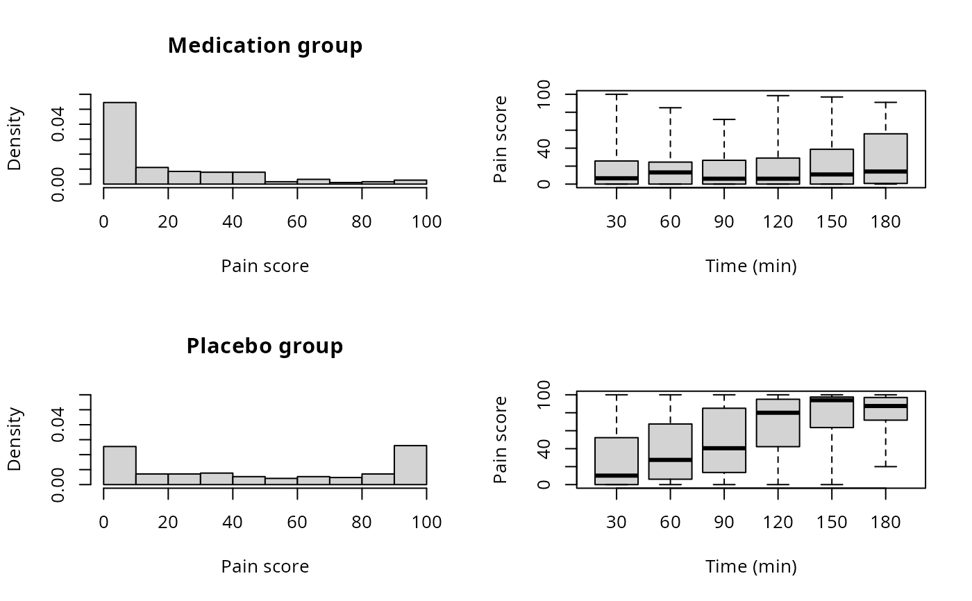
par(mfrow = c(2,2))

cx.lab <- 1
cx.ax <- 2.5
cx <- 2.5
yl <- c(0,0.06)

hist(new$y[new$treatment == 1], xlab = "Pain score", main = "Medication group",
  freq = FALSE, ylim = yl)

plot(y ~ x_gr, new, subset = new$treatment == 1, xlab = "Time (min)",
  ylab = "Pain score", axes = FALSE, range = 0)
axis(1, at = 1:6, labels = c(0:5)*30 + 30)
axis(2)
box()

hist(new$y[new$treatment == 0], xlab = "Pain score", main = "Placebo group",
  freq = FALSE, ylim = yl)

plot(y ~ x_gr, new, subset = new$treatment == 0, xlab = "Time (min)",
  ylab = "Pain score", axes = FALSE, range = 0)
axis(1, at = 1:6, labels = (0:5)*30 + 30)
axis(2)
box()


#

if (FALSE) { # \dontrun{

taus <- c(1:3/4)
ls <- seq(0,3.5,by=0.1)

fit.aos <- tsrq(y ~ x*treatment, data = new, tsf = "ao", symm = TRUE,
  dbounded = TRUE, tau = taus, lambda = ls)
fit.aoa <- tsrq(y ~ x*treatment, data = new, tsf = "ao", symm = FALSE,
  dbounded = TRUE, tau = taus, lambda = ls)
fit.mcjs <- tsrq(y ~ x*treatment, data = new, tsf = "mcjI", symm = TRUE,
  dbounded = TRUE, tau = taus, lambda = ls)
fit.mcja <- tsrq(y ~ x*treatment, data = new, tsf = "mcjI", symm = FALSE,
  dbounded = TRUE, tau = taus, lambda = ls)
fit.mcj2 <- tsrq2(y ~ x*treatment, data = new, dbounded = TRUE, tau = taus,
  lambda = seq(0,2,by=0.1), delta = seq(0,1.5,by=0.3))
fit.nlrq <- nlrq2(y ~ x*treatment, data = new, start = coef(fit.mcj2, all = TRUE)[,1],
  dbounded = TRUE, tau = taus)

sel <- 0 # placebo (change to sel == 1 for medication group)
x <- new$x
nd <- data.frame(x = seq(min(x), max(x), length=200), treatment = sel)
xx <- nd$x+1

par(mfrow = c(2,2))

fit <- fit.aos
yhat <- predict(fit, newdata = nd)

plot(y ~ x_gr, new, subset = new$treatment == sel, xlab = "",
  ylab = "Pain score", axes = FALSE, main = "Aranda-Ordaz (s)",
  range = 0, col = grey(4/5))
apply(yhat, 2, function(y,x) lines(x, y, lwd = 2), x = xx)
axis(1, at = 1:6, labels = (0:5)*30 + 30)
axis(2, at = c(0, 25, 50, 75, 100))
box()

fit <- fit.aoa
yhat <- predict(fit, newdata = nd)

plot(y ~ x_gr, new, subset = new$treatment == sel, xlab = "", ylab = "",
  axes = FALSE, main = "Aranda-Ordaz (a)", range = 0, col = grey(4/5))
apply(yhat, 2, function(y,x) lines(x, y, lwd = 2), x = xx)
axis(1, at = 1:6, labels = (0:5)*30 + 30)
axis(2, at = c(0, 25, 50, 75, 100))
box()

fit <- fit.mcjs
yhat <- predict(fit, newdata = nd)

plot(y ~ x_gr, new, subset = new$treatment == sel, xlab = "Time (min)",
  ylab = "Pain score", axes = FALSE, main = "Proposal I (s)",
  range = 0, col = grey(4/5))
apply(yhat, 2, function(y,x) lines(x, y, lwd = 2), x = xx)
axis(1, at = 1:6, labels = (0:5)*30 + 30)
axis(2, at = c(0, 25, 50, 75, 100))
box()

fit <- fit.mcj2
yhat <- predict(fit, newdata = nd)

plot(y ~ x_gr, new, subset = new$treatment == sel, xlab = "Time (min)",
  ylab = "", axes = FALSE, main = "Proposal II", range = 0, col = grey(4/5))
apply(yhat, 2, function(y,x) lines(x, y, lwd = 2), x = xx)
axis(1, at = 1:6, labels = (0:5)*30 + 30)
axis(2, at = c(0, 25, 50, 75, 100))
box()
} # }