Simulate fractional ARIMA Time Series

Generates simulated long-memory time series data from the fractional ARIMA(p,d,q) model. This is a test problem generator for fracdiff.

Note that the MA coefficients have inverted signs compared to other parametrizations, see the details in fracdiff.

Usage

fracdiff.sim(n, ar = NULL, ma = NULL, d,
             rand.gen = rnorm, innov = rand.gen(n+q, ...),
             n.start = NA, backComp = TRUE, allow.0.nstart = FALSE,
             start.innov = rand.gen(n.start, ...),
             ..., mu = 0)

Arguments

n: length of the time series.
ar: vector of autoregressive parameters; empty by default.
ma: vector of moving average parameters; empty by default.
d: fractional differencing parameter.
rand.gen: a function to generate the innovations; the default, rnorm generates white N(0,1) noise.
innov: an optional times series of innovations. If not provided, rand.gen() is used.
n.start: length of “burn-in” period. If NA, the default, the same value as in arima.sim is computed.
backComp: logical indicating if back compatibility with older versions of fracdiff.sim is desired. Otherwise, for d = 0, compatibility with R's arima.sim is achieved.
allow.0.nstart: logical indicating if n.start = 0 should be allowed even when \(p + q > 0\). This not recommended unless for producing the same series as with older versions of fracdiff.sim.
start.innov: an optional vector of innovations to be used for the burn-in period. If supplied there must be at least n.start values.
...: additional arguments for rand.gen(). Most usefully, the standard deviation of the innovations generated by rnorm can be specified by sd.
mu: time series mean (added at the end).

Value

a list containing the following elements :

series: time series
ar, ma, d, mu, n.start: same as input

Examples

## Pretty (too) short to "see" the long memory
fracdiff.sim(100, ar = .2, ma = .4, d = .3)
#> $series
#>   [1] -0.54508854  0.12211067 -0.87249044  0.62846848  0.52773081 -0.79149130
#>   [7] -0.35577461  0.16736432 -1.57945501 -0.14568874  0.68102186  2.82731531
#>  [13]  0.81575745  0.57655192  0.04488837  2.18015672  1.50388559  1.34775187
#>  [19] -0.65015788  0.93544850  2.67082263  1.22781823  0.77662506  2.24341859
#>  [25]  1.06144512  0.97916765 -0.40567809  1.90069450  1.45486955  0.47967942
#>  [31]  2.14969819 -0.62202961 -0.17976417  0.61891035  2.65965317  1.82092913
#>  [37]  0.56590219  1.40207818  1.61168847  1.98300062  1.17307260  1.31872386
#>  [43]  1.40930069  0.22337605  0.80336167  0.89643405  0.52472357  0.51986329
#>  [49]  0.21587905  0.57230979  1.39493233  1.28486610  1.23836496  1.24947598
#>  [55]  1.68645810  1.08584110  1.67114544  1.76873326  1.29250849  1.98420212
#>  [61]  0.12583463 -0.40096997 -0.75329888 -0.50362579  0.76049923  0.08338284
#>  [67]  1.83551068  0.20172165  0.05776280  1.00581661  0.49019420 -1.68332580
#>  [73] -1.36683146 -0.85870661 -0.14061598 -0.18422388  1.54744921  1.01468453
#>  [79] -1.18123161 -0.31106128  0.04865101  0.29270234  0.66807957 -0.85893971
#>  [85]  0.05347749  0.86009046 -1.12522122 -0.36252565  1.14808186 -0.95977101
#>  [91]  0.90859504 -0.09608575 -0.70697921  1.07880821  0.88311782  0.51961325
#>  [97]  0.77022683 -1.19208274 -0.11825963 -0.31193450
#> 
#> $ar
#> [1] 0.2
#> 
#> $ma
#> [1] 0.4
#> 
#> $d
#> [1] 0.3
#> 
#> $mu
#> [1] 0
#> 
#> $n.start
#> [1] 6
#> 

## longer with "extreme" ar:
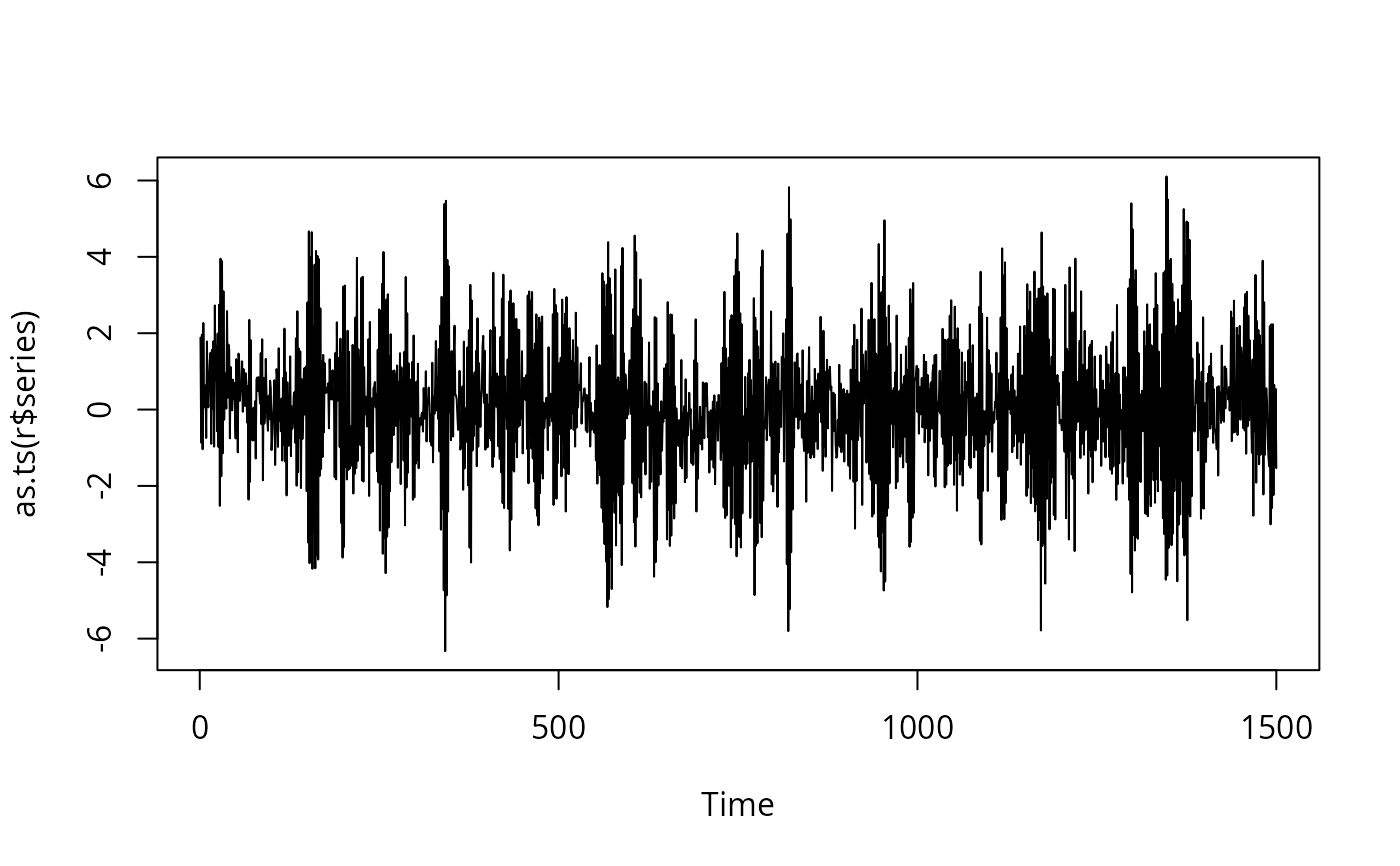
r <- fracdiff.sim(n=1500, ar=-0.9, d= 0.3)
plot(as.ts(r$series))


## Show that  MA  coefficients meaning is inverted
## compared to   stats :: arima :

AR <- 0.7
MA <- -0.5
n.st <- 2

AR <- c(0.7, -0.1)
MA <- c(-0.5, 0.4)
n <- 512 ; sd <- 0.1
n.st <- 10

set.seed(101)
Y1 <- arima.sim(list(ar = AR, ma = MA), n = n, n.start = n.st, sd = sd)
plot(Y1)

# For our fracdiff, reverse the MA sign:
set.seed(101)
Y2 <- fracdiff.sim(n = n, ar = AR, ma = - MA, d = 0,
                   n.start = n.st, sd = sd)$series
lines(Y2, col=adjustcolor("red", 0.5))

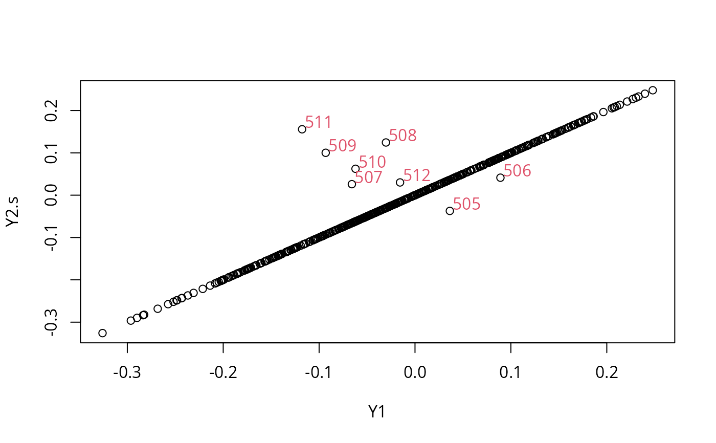
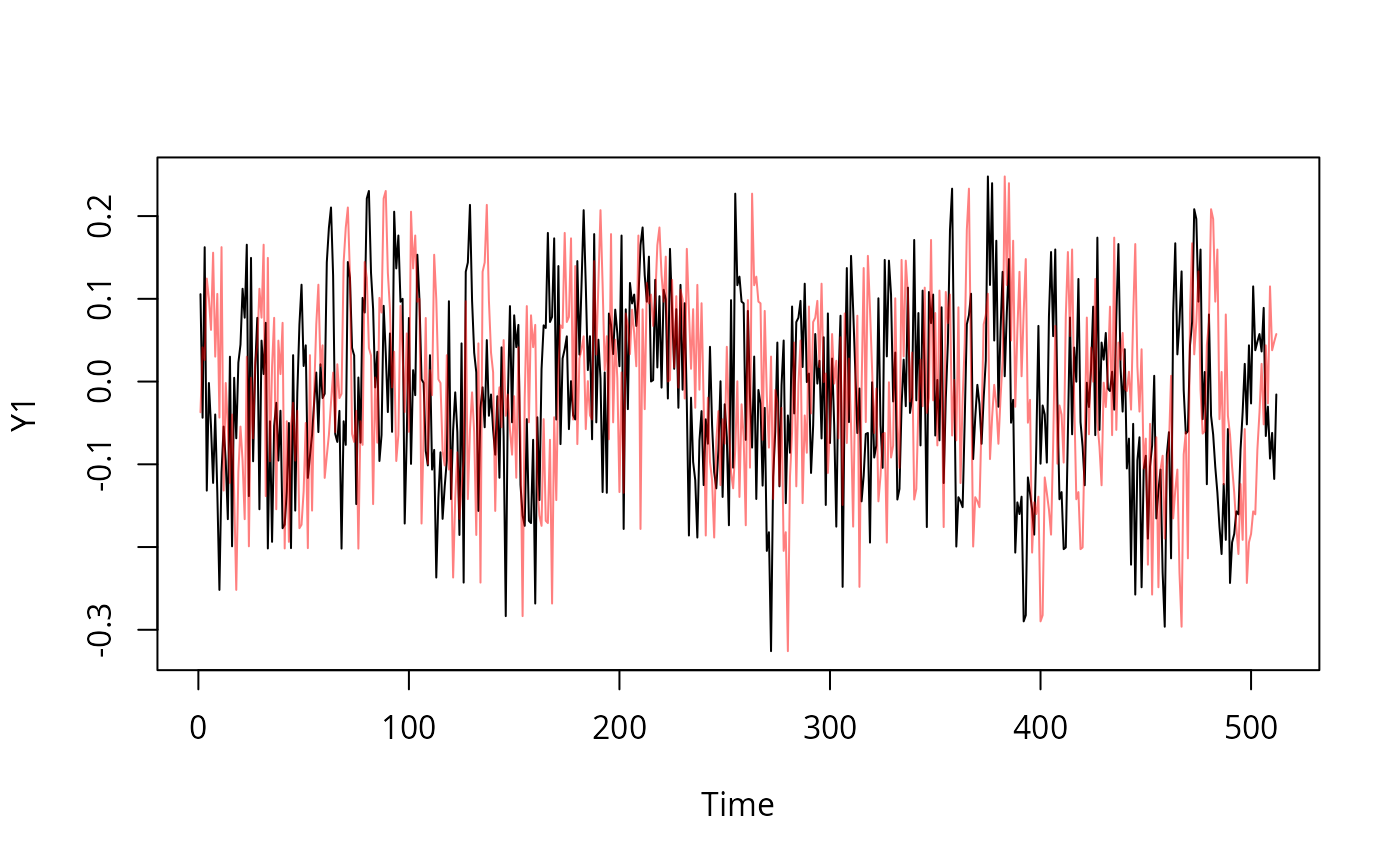## .. no, you don't need glasses ;-)  Y2 is Y1 shifted slightly

##' rotate left by k (k < 0: rotate right)
rot <- function(x, k) {
  stopifnot(k == round(k))
  n <- length(x)
  if(k <- k %% n) x[c((k+1):n, 1:k)] else x
}
k <- n.st - 2
Y2.s <- rot(Y2, k)
head.matrix(cbind(Y1, Y2.s))
#>                Y1         Y2.s
#> [1,]  0.105653840  0.105986817
#> [2,] -0.043723547 -0.043557047
#> [3,]  0.162403833  0.162487085
#> [4,] -0.131808486 -0.131766860
#> [5,] -0.001723455 -0.001702642
#> [6,] -0.054197985 -0.054187579
plot(Y1, Y2.s); i <- (n-k+1):n
text(Y1[i], Y2.s[i], i, adj = c(0,0)-.1, col=2)


## With  backComp = FALSE,  get *the same* as arima.sim():
set.seed(101)
Y2. <- fracdiff.sim(n = n, ar = AR, ma = - MA, d = 0,
                    n.start = n.st, sd = sd, backComp = FALSE)$series
stopifnot( all.equal( c(Y1), Y2., tolerance= 1e-15))

Usage

Arguments

Value

See also

Examples