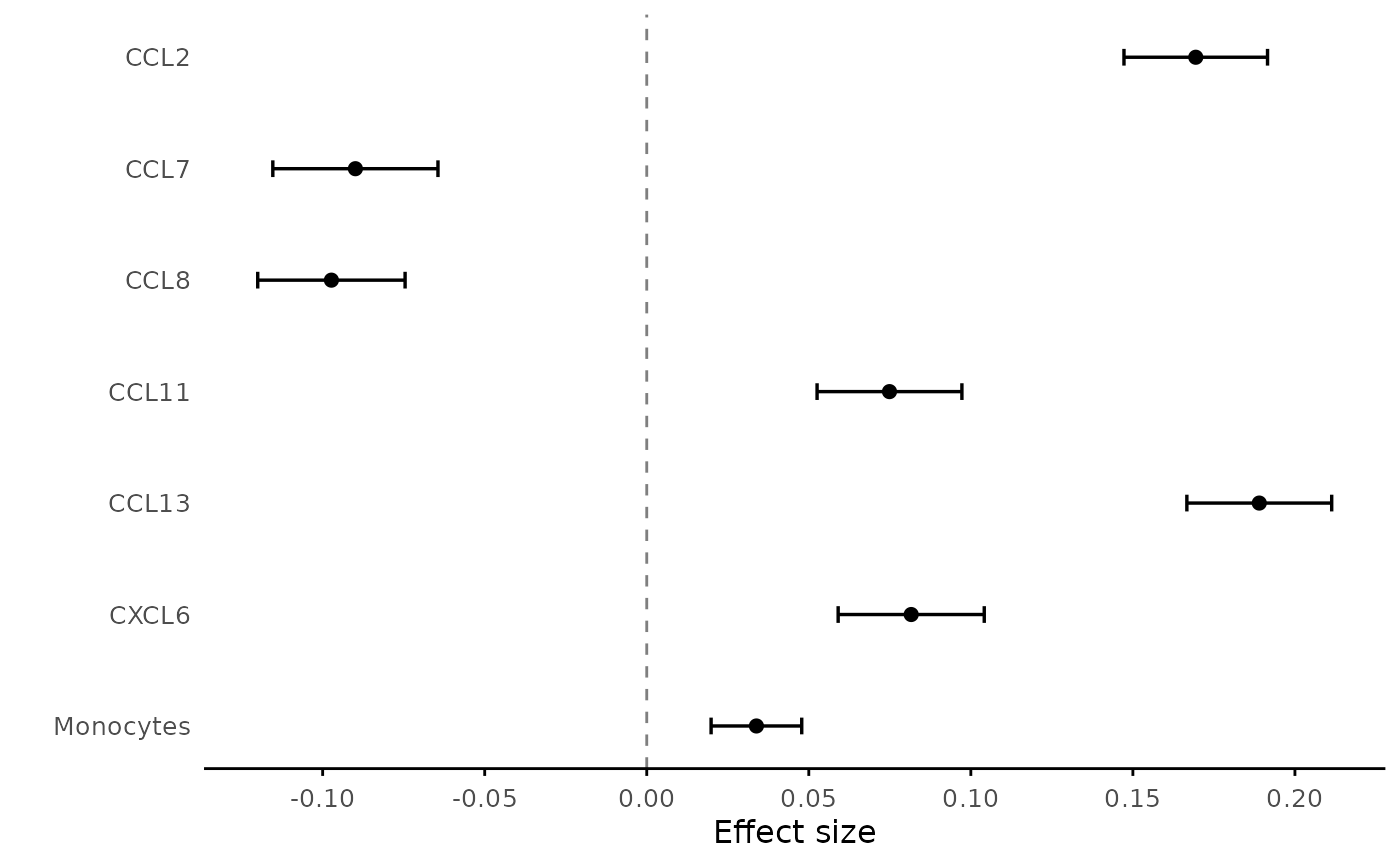
The function accepts parameter estimates and their standard errors from one or more models and produces a horizontal forest plot with confidence intervals.
Two plotting modes are supported:
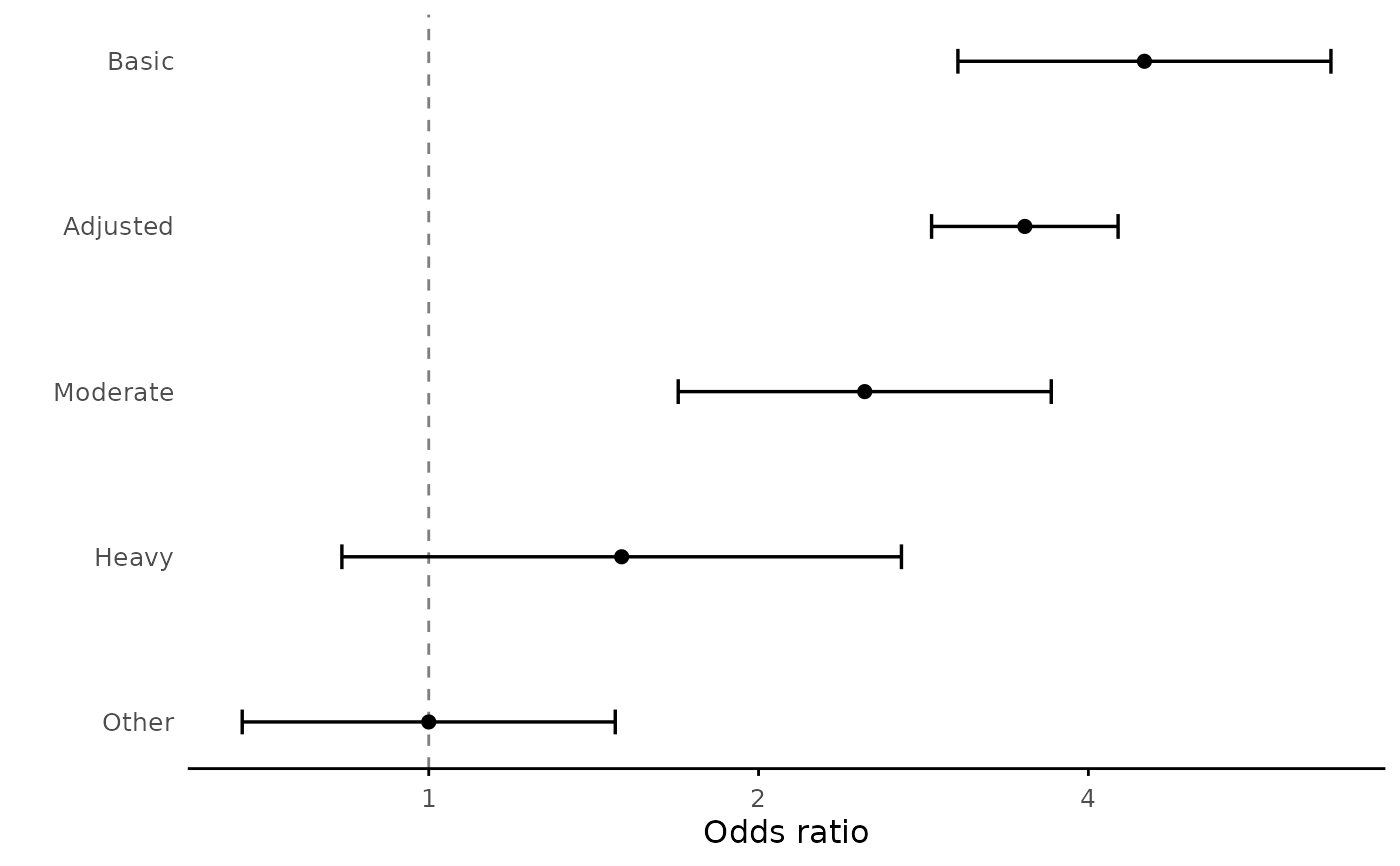
transform="none"(default): plots estimates on the linear scale (typical for GWAS or Mendelian randomisation beta coefficients).transform="exp": plots exponentiated estimates on a log10 axis (typical for odds ratios or hazard ratios). Confidence intervals are computed on the log scale and back-transformed.
Usage
ESplot(
  ESdat,
  alpha = 0.05,
  fontsize = 12,
  transform = c("none", "exp"),
  xlab = NULL
)
Arguments
- ESdat
Data frame with three columns:
id Model or trait label
b Effect estimate (beta or log(OR)/log(HR))
se Standard error of the estimate
- alpha
Type-I error rate for the confidence interval (default 0.05 for 95% CI).
- fontsize
Base font size used in the plot.
- transform
Either
"none"(linear scale) or"exp"(exponentiated scale).- xlab
Optional x-axis label. If
NULL, a sensible default is used.
Details
Create a publication-ready forest plot for model effect estimates. The function supports both linear effect sizes (e.g. regression betas) and exponentiated effects (e.g. odds ratios or hazard ratios).
Confidence intervals are computed as $$ estimate \pm z_{\alpha/2} \times SE $$
When transform="exp", estimates are interpreted as log(OR) or log(HR)
and are exponentiated before plotting. The x-axis is displayed on a
log10 scale and the reference line is placed at 1.
This function replaces an earlier base-R implementation and provides a consistent interface for GWAS, Mendelian randomisation, and epidemiological regression analyses.
Examples
## Example 1: Linear effect sizes (GWAS / MR)
rs12075 <- data.frame(
id=c("CCL2","CCL7","CCL8","CCL11","CCL13","CXCL6","Monocytes"),
b=c(0.1694,-0.0899,-0.0973,0.0749,0.189,0.0816,0.0338387),
se=c(0.0113,0.013,0.0116,0.0114,0.0114,0.0115,0.00713386)
)
ESplot(rs12075)
 ## Example 2: Odds ratios
dat <- data.frame(
id=c("Basic","Adjusted","Moderate","Heavy","Other"),
b=log(c(4.5,3.5,2.5,1.5,1)),
se=c(0.2,0.1,0.2,0.3,0.2)
)
ESplot(dat, transform="exp")
## Example 2: Odds ratios
dat <- data.frame(
id=c("Basic","Adjusted","Moderate","Heavy","Other"),
b=log(c(4.5,3.5,2.5,1.5,1)),
se=c(0.2,0.1,0.2,0.3,0.2)
)
ESplot(dat, transform="exp")