Predicted values are computed and, by default, plotted as a band plus an
optional line within. stat_quant_band() supports the use of both
x and y as explanatory variable in the model formula.
Usage
stat_quant_band(
  mapping = NULL,
  data = NULL,
  geom = "smooth",
  position = "identity",
  ...,
  quantiles = c(0.25, 0.5, 0.75),
  formula = NULL,
  fit.seed = NA,
  fm.values = FALSE,
  n = 80,
  method = "rq",
  method.args = list(),
  n.min = 3L,
  na.rm = FALSE,
  orientation = NA,
  show.legend = NA,
  inherit.aes = TRUE
)
Arguments
- mapping
The aesthetic mapping, usually constructed with
aes. Only needs to be set at the layer level if you are overriding the plot defaults.- data
A layer specific dataset, only needed if you want to override the plot defaults.
- geom
The geometric object to use display the data
- position
The position adjustment to use for overlapping points on this layer.
- ...
other arguments passed on to
layer. This can include aesthetics whose values you want to set, not map. Seelayerfor more details.- quantiles
A numeric vector of length 3, with unique values in \(0\ldots 1\). The three quantile regressions are mapped to
y,ymaxandyminaesthetics, and by default plotted as a line and band.- formula
a formula object. Using aesthetic names
xandyinstead of original variable names.- fit.seed
RNG seed argument passed to
set.seed(). Defaults toNA, indicating thatset.seed()should not be called.- fm.values
logical Add metadata and parameter estimates extracted from the fitted model object;
FALSEby default.- n
Number of points at which to predict with the fitted model.
- method
function or character If character, "rq", "rqss" or the name of a model fit function are accepted, possibly followed by the fit function's
methodargument separated by a colon (e.g."rq:br"). If a function different torq(), it must accept arguments namedformula,data,weights,tauandmethodand return a model fit object of classrq,rqsorrqss.- method.args
named list with additional arguments passed to
rq(),rqss()or to another function passed as argument tomethod.- n.min
integer Minimum number of distinct values in the explanatory variable (on the rhs of formula) for fitting to the attempted.
- na.rm
a logical indicating whether NA values should be stripped before the computation proceeds.
- orientation
character Either "x" or "y" controlling the default for
formula. The letter indicates the aesthetic considered the explanatory variable in the model fit.- show.legend
logical. Should this layer be included in the legends?
NA, the default, includes if any aesthetics are mapped.FALSEnever includes, andTRUEalways includes.- inherit.aes
If
FALSE, overrides the default aesthetics, rather than combining with them. This is most useful for helper functions that define both data and aesthetics and shouldn't inherit behaviour from the default plot specification, e.g.borders.
Value
The value returned by the statistic is a data frame, that will have
n rows of predicted values for three quantiles as y,
ymin and ymax, plus x.
Details
This statistic is similar to stat_quant_line but plots the
quantiles differently with the band representing a region between two
quantiles, while in stat_quant_line() the bands plotted when
se = TRUE represent confidence intervals for the fitted quantile
lines.
geom_smooth, which is used by default, treats each
axis differently and thus is dependent on orientation. If no argument is
passed to formula, it defaults to y ~ x but x ~y is also
accepted, and equivalent to y ~ x plus orientation = "y".
Package 'ggpmisc' does not define a new geometry matching this statistic as
it is enough for the statistic to return suitable `x` and `y` values.
Aesthetics
stat_quant_eq expects x and y,
aesthetics to be used in the formula rather than the names of the
variables mapped to them. If present, the variable mapped to the
weight aesthetics is passed as argument to parameter weights
of the fitting function. All three must be mapped to numeric
variables. In addition, the aesthetics recognized by the geometry
("geom_smooth" is the default) are obeyed and grouping
respected.
See also
Other ggplot statistics for quantile regression:
stat_quant_eq(),
stat_quant_line()
Examples
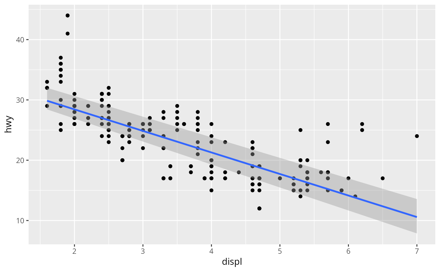
ggplot(mpg, aes(displ, hwy)) +
geom_point() +
stat_quant_band()
 # If you need the fitting to be done along the y-axis set the orientation
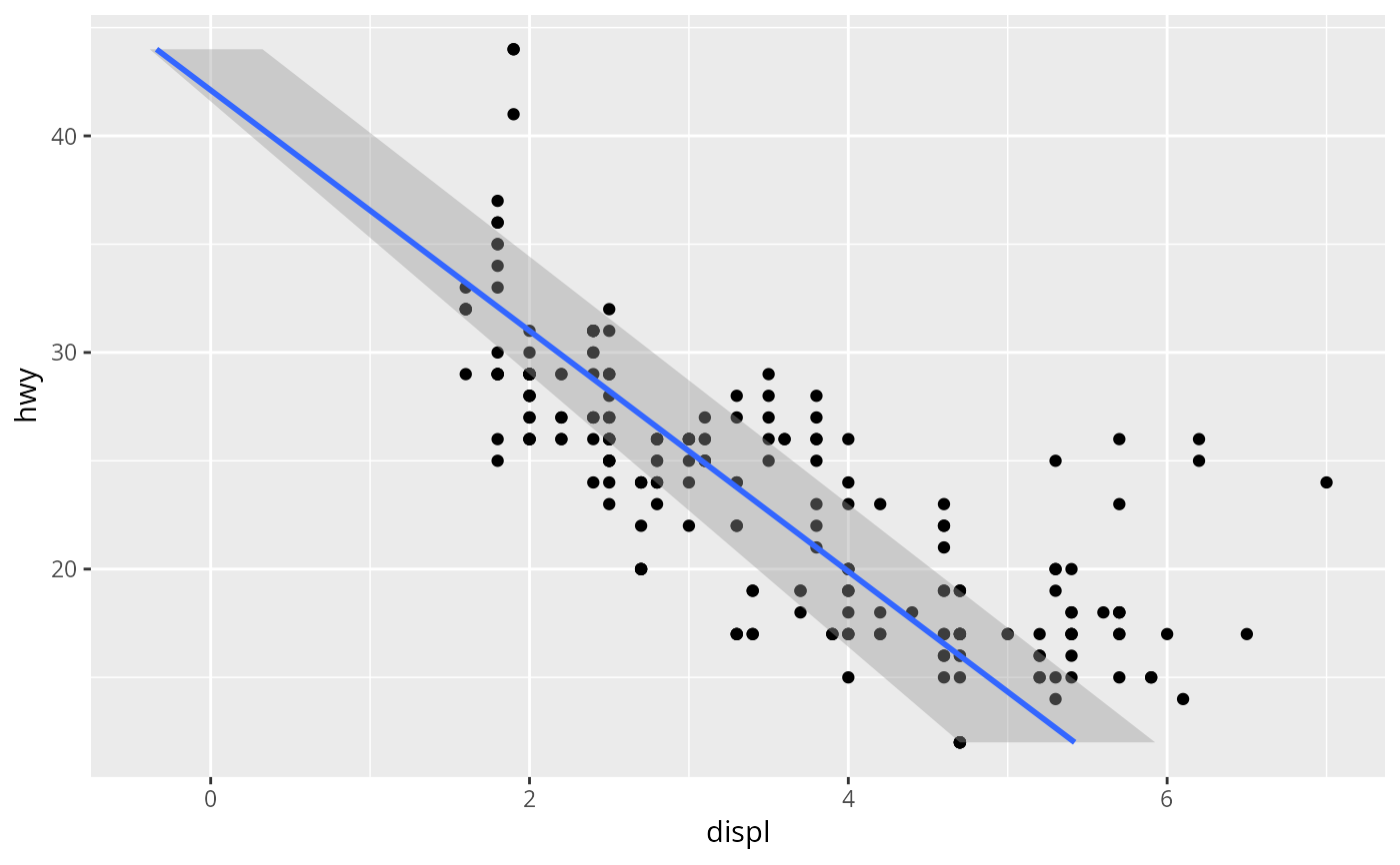
ggplot(mpg, aes(displ, hwy)) +
geom_point() +
stat_quant_band(orientation = "y")
# If you need the fitting to be done along the y-axis set the orientation
ggplot(mpg, aes(displ, hwy)) +
geom_point() +
stat_quant_band(orientation = "y")
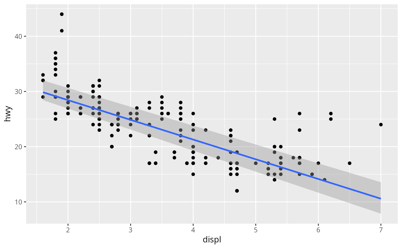
 ggplot(mpg, aes(displ, hwy)) +
geom_point() +
stat_quant_band(formula = y ~ x)
ggplot(mpg, aes(displ, hwy)) +
geom_point() +
stat_quant_band(formula = y ~ x)
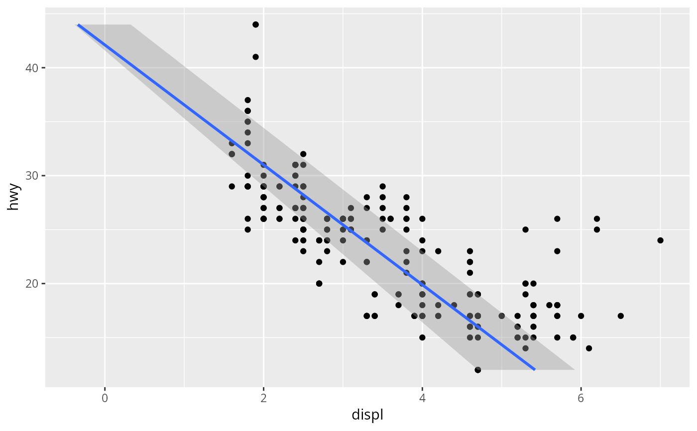
 ggplot(mpg, aes(displ, hwy)) +
geom_point() +
stat_quant_band(formula = x ~ y)
ggplot(mpg, aes(displ, hwy)) +
geom_point() +
stat_quant_band(formula = x ~ y)
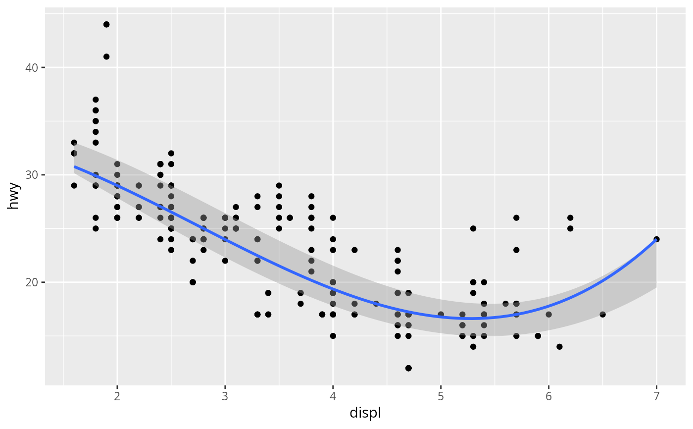
 ggplot(mpg, aes(displ, hwy)) +
geom_point() +
stat_quant_band(formula = y ~ poly(x, 3))
ggplot(mpg, aes(displ, hwy)) +
geom_point() +
stat_quant_band(formula = y ~ poly(x, 3))
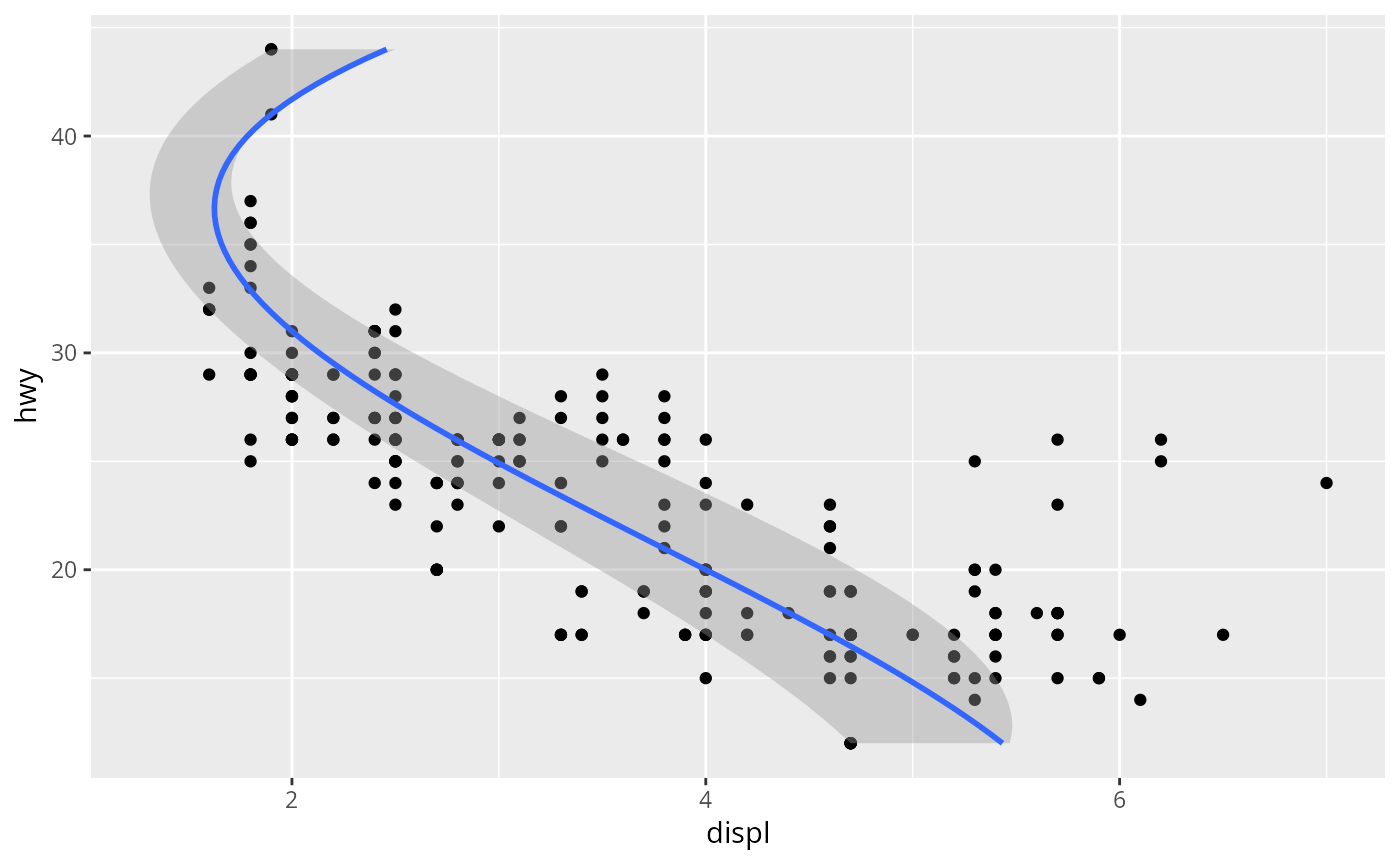
 ggplot(mpg, aes(displ, hwy)) +
geom_point() +
stat_quant_band(formula = x ~ poly(y, 3))
ggplot(mpg, aes(displ, hwy)) +
geom_point() +
stat_quant_band(formula = x ~ poly(y, 3))
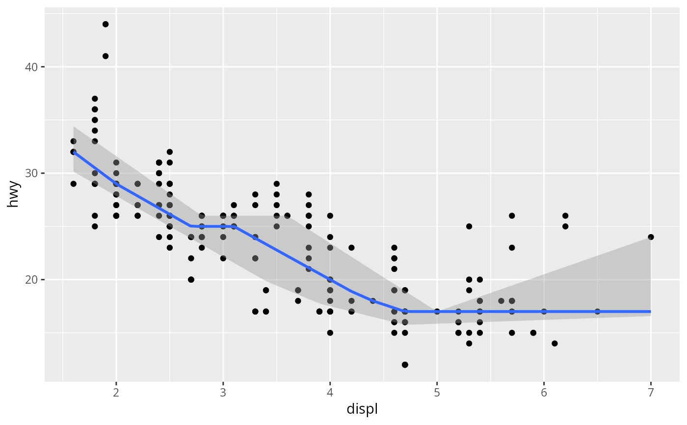
 # Instead of rq() we can use rqss() to fit an additive model:
ggplot(mpg, aes(displ, hwy)) +
geom_point() +
stat_quant_band(method = "rqss",
formula = y ~ qss(x))
# Instead of rq() we can use rqss() to fit an additive model:
ggplot(mpg, aes(displ, hwy)) +
geom_point() +
stat_quant_band(method = "rqss",
formula = y ~ qss(x))
 ggplot(mpg, aes(displ, hwy)) +
geom_point() +
stat_quant_band(method = "rqss",
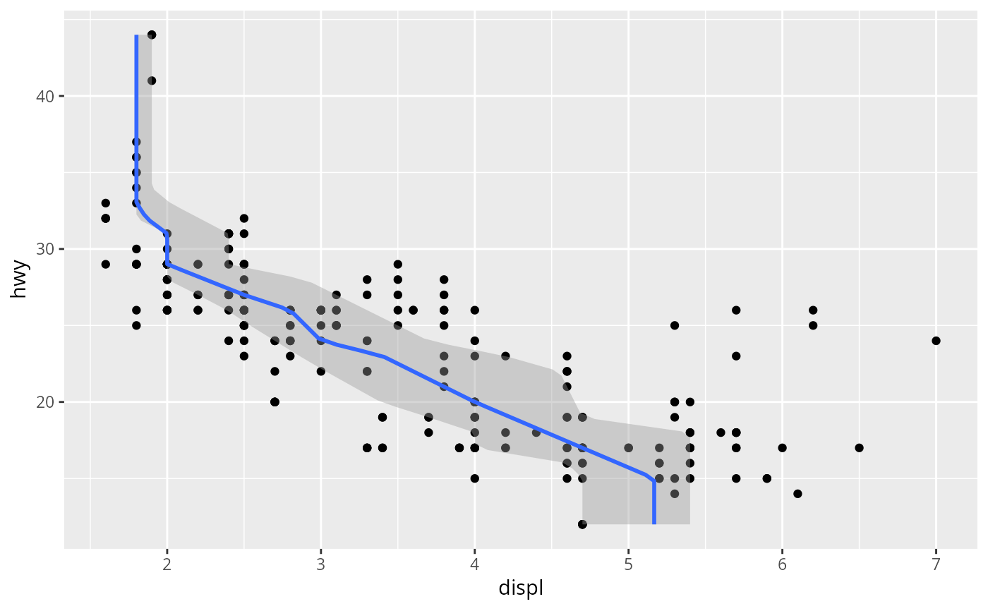
formula = x ~ qss(y, constraint = "D"))
ggplot(mpg, aes(displ, hwy)) +
geom_point() +
stat_quant_band(method = "rqss",
formula = x ~ qss(y, constraint = "D"))
 # Regressions are automatically fit to each group (defined by categorical
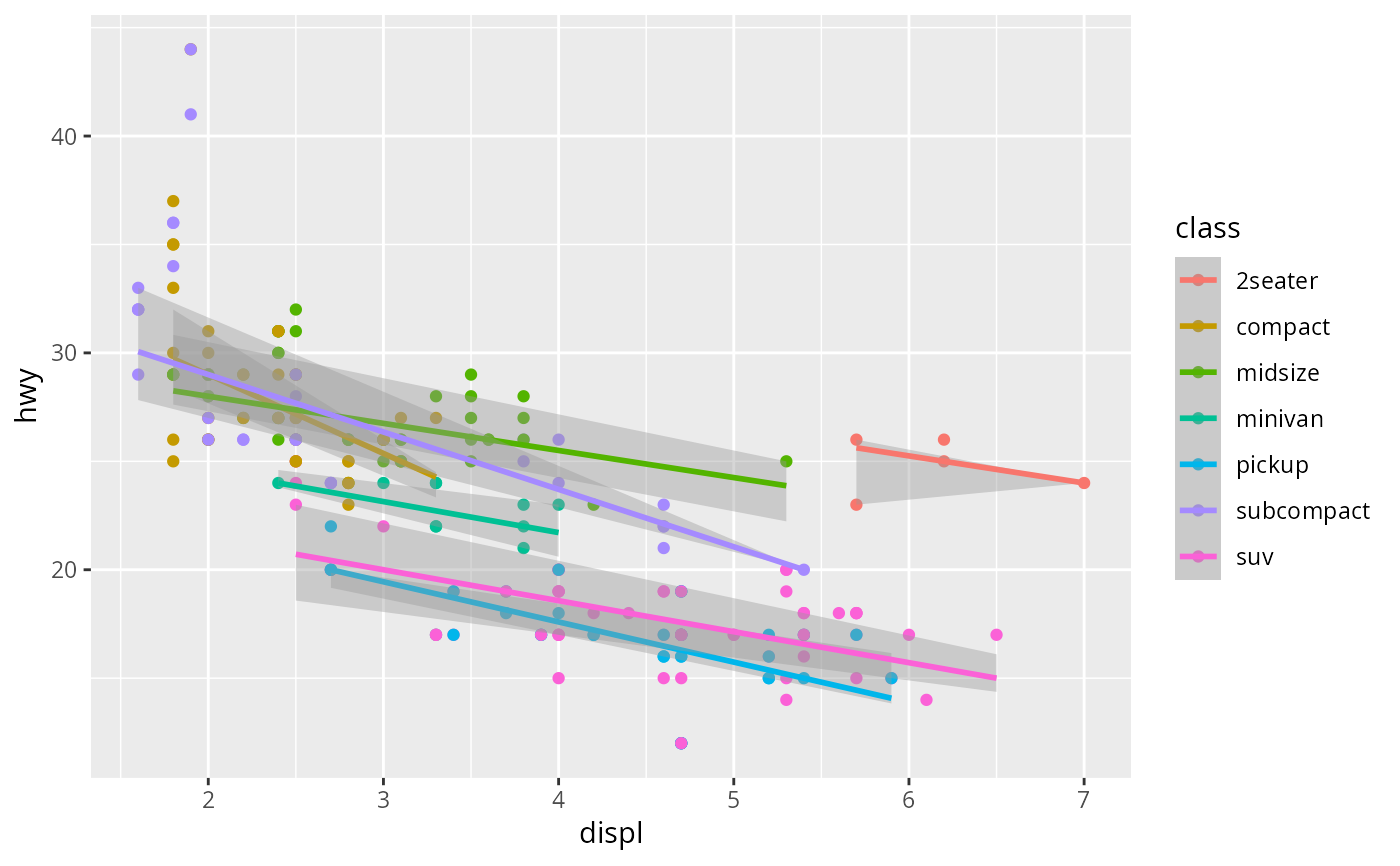
# aesthetics or the group aesthetic) and for each facet.
ggplot(mpg, aes(displ, hwy, colour = class)) +
geom_point() +
stat_quant_band(formula = y ~ x)
#> Warning: Solution may be nonunique
#> Warning: Solution may be nonunique
# Regressions are automatically fit to each group (defined by categorical
# aesthetics or the group aesthetic) and for each facet.
ggplot(mpg, aes(displ, hwy, colour = class)) +
geom_point() +
stat_quant_band(formula = y ~ x)
#> Warning: Solution may be nonunique
#> Warning: Solution may be nonunique
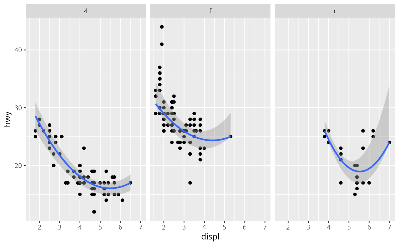
 ggplot(mpg, aes(displ, hwy)) +
geom_point() +
stat_quant_band(formula = y ~ poly(x, 2)) +
facet_wrap(~drv)
ggplot(mpg, aes(displ, hwy)) +
geom_point() +
stat_quant_band(formula = y ~ poly(x, 2)) +
facet_wrap(~drv)
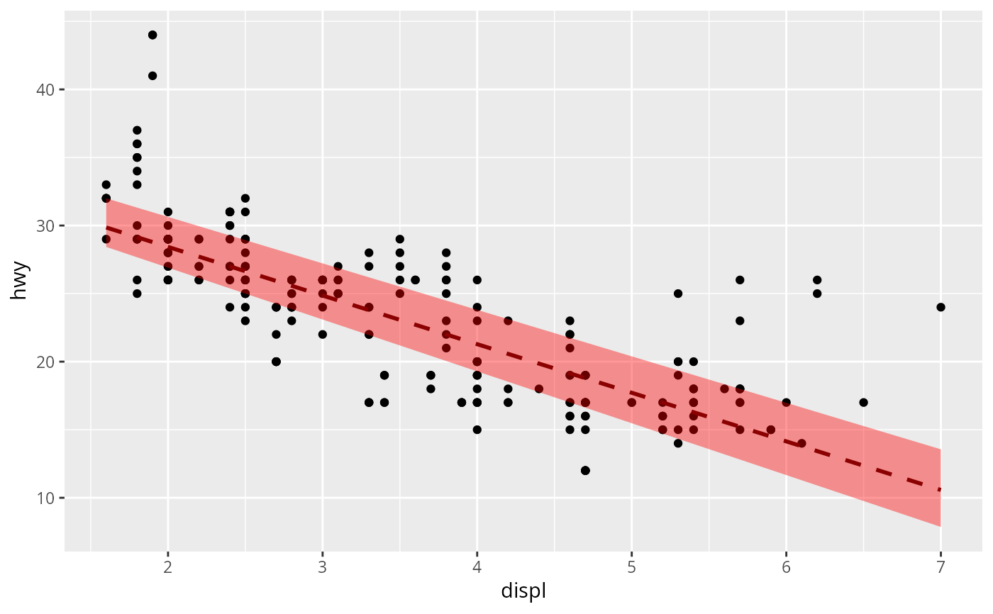
 ggplot(mpg, aes(displ, hwy)) +
geom_point() +
stat_quant_band(linetype = "dashed", color = "darkred", fill = "red")
ggplot(mpg, aes(displ, hwy)) +
geom_point() +
stat_quant_band(linetype = "dashed", color = "darkred", fill = "red")
 ggplot(mpg, aes(displ, hwy)) +
stat_quant_band(color = NA, alpha = 1) +
geom_point()
ggplot(mpg, aes(displ, hwy)) +
stat_quant_band(color = NA, alpha = 1) +
geom_point()
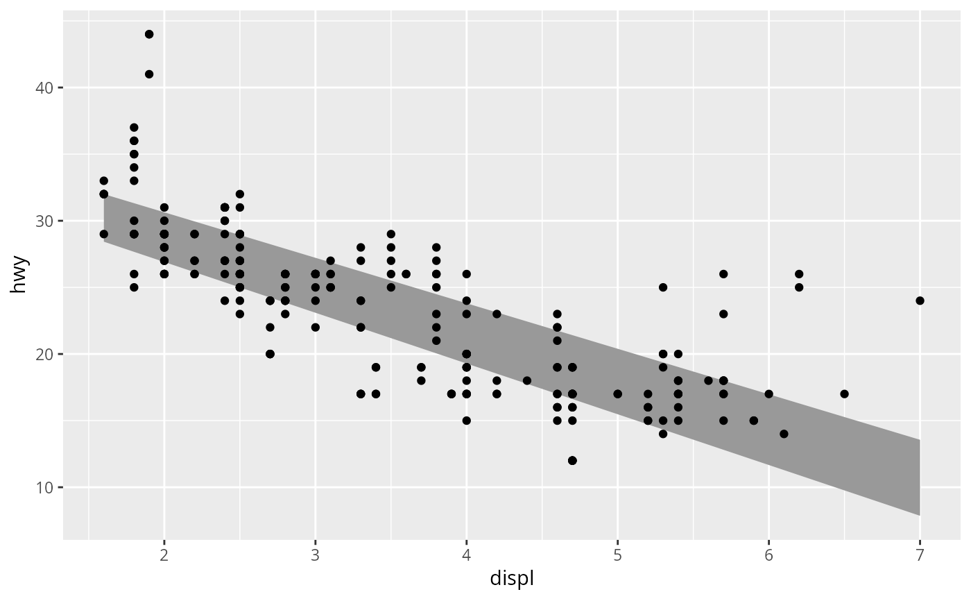 ggplot(mpg, aes(displ, hwy)) +
stat_quant_band(quantiles = c(0, 0.1, 0.2)) +
geom_point()
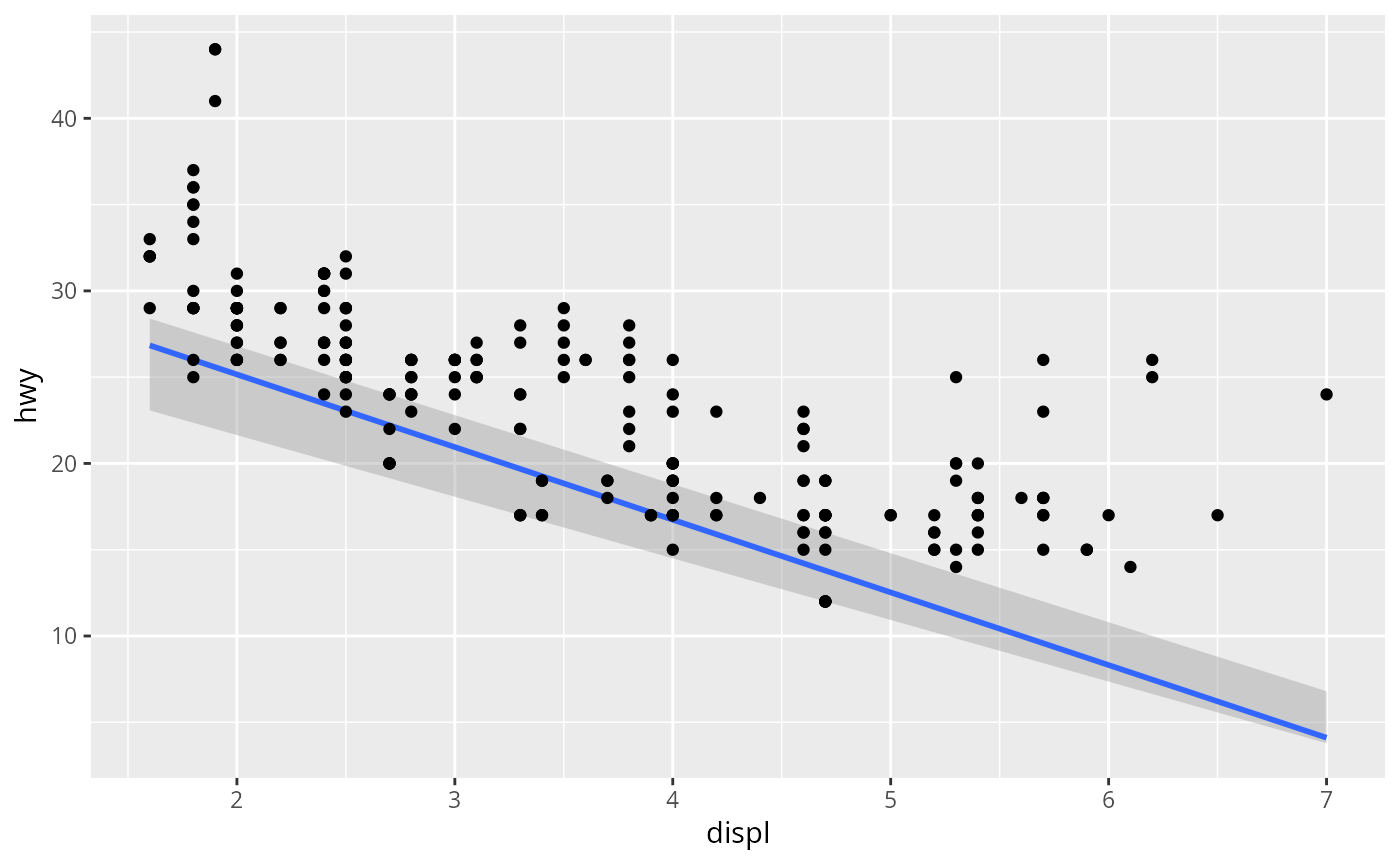
ggplot(mpg, aes(displ, hwy)) +
stat_quant_band(quantiles = c(0, 0.1, 0.2)) +
geom_point()
 # Inspecting the returned data using geom_debug()
gginnards.installed <- requireNamespace("gginnards", quietly = TRUE)
if (gginnards.installed)
library(gginnards)
if (gginnards.installed)
ggplot(mpg, aes(displ, hwy)) +
stat_quant_band(geom = "debug")
#> Warning: Ignoring unknown parameters: `se`
# Inspecting the returned data using geom_debug()
gginnards.installed <- requireNamespace("gginnards", quietly = TRUE)
if (gginnards.installed)
library(gginnards)
if (gginnards.installed)
ggplot(mpg, aes(displ, hwy)) +
stat_quant_band(geom = "debug")
#> Warning: Ignoring unknown parameters: `se`
 #> [1] "PANEL 1; group(s) -1; 'draw_function()' input 'data' (head):"
#> x ymin y ymax flipped_aes PANEL group orientation
#> 1 1.600000 28.42857 29.85714 32.00000 FALSE 1 -1 x
#> 2 1.668354 28.16817 29.61302 31.76659 FALSE 1 -1 x
#> 3 1.736709 27.90778 29.36890 31.53319 FALSE 1 -1 x
#> 4 1.805063 27.64738 29.12477 31.29978 FALSE 1 -1 x
#> 5 1.873418 27.38698 28.88065 31.06638 FALSE 1 -1 x
#> 6 1.941772 27.12658 28.63653 30.83297 FALSE 1 -1 x
if (gginnards.installed)
ggplot(mpg, aes(displ, hwy)) +
stat_quant_band(geom = "debug", fm.values = TRUE)
#> Warning: Ignoring unknown parameters: `se`
#> [1] "PANEL 1; group(s) -1; 'draw_function()' input 'data' (head):"
#> x ymin y ymax flipped_aes PANEL group orientation
#> 1 1.600000 28.42857 29.85714 32.00000 FALSE 1 -1 x
#> 2 1.668354 28.16817 29.61302 31.76659 FALSE 1 -1 x
#> 3 1.736709 27.90778 29.36890 31.53319 FALSE 1 -1 x
#> 4 1.805063 27.64738 29.12477 31.29978 FALSE 1 -1 x
#> 5 1.873418 27.38698 28.88065 31.06638 FALSE 1 -1 x
#> 6 1.941772 27.12658 28.63653 30.83297 FALSE 1 -1 x
if (gginnards.installed)
ggplot(mpg, aes(displ, hwy)) +
stat_quant_band(geom = "debug", fm.values = TRUE)
#> Warning: Ignoring unknown parameters: `se`
 #> [1] "PANEL 1; group(s) -1; 'draw_function()' input 'data' (head):"
#> x ymin fm1.class fm1.formula.chr y fm2.class
#> 1 1.600000 28.42857 rq y ~ x 29.85714 rq
#> 2 1.668354 28.16817 rq y ~ x 29.61302 rq
#> 3 1.736709 27.90778 rq y ~ x 29.36890 rq
#> 4 1.805063 27.64738 rq y ~ x 29.12477 rq
#> 5 1.873418 27.38698 rq y ~ x 28.88065 rq
#> 6 1.941772 27.12658 rq y ~ x 28.63653 rq
#> fm2.formula.chr ymax fm3.class fm3.formula.chr n fm.method flipped_aes
#> 1 y ~ x 32.00000 rq y ~ x 234 rq FALSE
#> 2 y ~ x 31.76659 rq y ~ x 234 rq FALSE
#> 3 y ~ x 31.53319 rq y ~ x 234 rq FALSE
#> 4 y ~ x 31.29978 rq y ~ x 234 rq FALSE
#> 5 y ~ x 31.06638 rq y ~ x 234 rq FALSE
#> 6 y ~ x 30.83297 rq y ~ x 234 rq FALSE
#> PANEL group orientation
#> 1 1 -1 x
#> 2 1 -1 x
#> 3 1 -1 x
#> 4 1 -1 x
#> 5 1 -1 x
#> 6 1 -1 x
#> [1] "PANEL 1; group(s) -1; 'draw_function()' input 'data' (head):"
#> x ymin fm1.class fm1.formula.chr y fm2.class
#> 1 1.600000 28.42857 rq y ~ x 29.85714 rq
#> 2 1.668354 28.16817 rq y ~ x 29.61302 rq
#> 3 1.736709 27.90778 rq y ~ x 29.36890 rq
#> 4 1.805063 27.64738 rq y ~ x 29.12477 rq
#> 5 1.873418 27.38698 rq y ~ x 28.88065 rq
#> 6 1.941772 27.12658 rq y ~ x 28.63653 rq
#> fm2.formula.chr ymax fm3.class fm3.formula.chr n fm.method flipped_aes
#> 1 y ~ x 32.00000 rq y ~ x 234 rq FALSE
#> 2 y ~ x 31.76659 rq y ~ x 234 rq FALSE
#> 3 y ~ x 31.53319 rq y ~ x 234 rq FALSE
#> 4 y ~ x 31.29978 rq y ~ x 234 rq FALSE
#> 5 y ~ x 31.06638 rq y ~ x 234 rq FALSE
#> 6 y ~ x 30.83297 rq y ~ x 234 rq FALSE
#> PANEL group orientation
#> 1 1 -1 x
#> 2 1 -1 x
#> 3 1 -1 x
#> 4 1 -1 x
#> 5 1 -1 x
#> 6 1 -1 x