Plotting Hexagon Cells with a Legend
gplot.hexbin.RdPlots Hexagons visualizing the counts in an hexbin object. Different styles are availables. Provides a legend indicating the count representations.
Usage
<!-- %% In future: No longer export   gplot.hexbin() ! -->
gplot.hexbin(x, style = "colorscale", legend = 1.2, lcex = 1,
      minarea = 0.04, maxarea = 0.8, mincnt = 1, maxcnt = max(x@count),
      trans = NULL, inv = NULL, colorcut = seq(0, 1, length = min(17, maxcnt)),
      border = NULL, density = NULL, pen = NULL,
      colramp = function(n) LinGray(n,beg = 90,end = 15),
      xlab = "", ylab = "", main = "", newpage = TRUE,
      type = c("p", "l", "n"), xaxt = c("s", "n"), yaxt = c("s", "n"),
      clip = "on", verbose = getOption("verbose"))
<!-- %% FIXME: This is the S4 plot method for 'hexbin' -->
<!-- %%        currently also exported "standalone" - for testing,debugging.. -->
<!-- %% we'd really don't want to repeat the argument list; use \synopsis{.} ? -->
# S4 method for class 'hexbin,missing'
plot(x, style = "colorscale", legend = 1.2, lcex = 1,
      minarea = 0.04, maxarea = 0.8, mincnt = 1, maxcnt = max(x@count),
      trans = NULL, inv = NULL, colorcut = seq(0, 1, length = min(17, maxcnt)),
      border = NULL, density = NULL, pen = NULL,
      colramp = function(n) LinGray(n,beg = 90,end = 15),
      xlab = "", ylab = "", main = "", newpage = TRUE,
      type = c("p", "l", "n"), xaxt = c("s", "n"), yaxt = c("s", "n"),
      clip = "on", verbose = getOption("verbose"))
Arguments
- x
an object of class
hexbin.
- style
string specifying the style of hexagon plot, see
grid.hexagonsfor the possibilities.- legend
numeric width of the legend in inches of
FALSE. In the latter case, or when0, no legend is not produced.- lcex
characters expansion size for the text in the legend
- minarea
fraction of cell area for the lowest count
- maxarea
fraction of the cell area for the largest count
- mincnt
cells with fewer counts are ignored.
- maxcnt
cells with more counts are ignored.
- trans
functionspecifying a transformation for the counts such assqrt.
- inv
the inverse transformation of
trans.- colorcut
vector of values covering [0, 1] that determine hexagon color class boundaries and hexagon legend size boundaries. Alternatively, an integer (
<= maxcnt) specifying the number of equispaced colorcut values in [0,1].- border, density, pen
color for polygon borders and filling of each hexagon drawn, passed to
grid.hexagons.- colramp
function accepting an integer
nas an argument and returning n colors.- xlab, ylab
x- and y-axis label.
- main
main title.
- newpage
should a new page start?.
- type, xaxt, yaxt
strings to be used (when set to
"n") for suppressing the plotting of hexagon symbols, or the x- or y-axis, respectively.- clip
either 'on' or 'off' are the allowed arguments, when on everything is clipped to the plotting region.
- verbose
logical indicating if some diagnostic output should happen.
Details
This is the (S4) plot method for hexbin (and
erodebin) objects (erodebin-class).
To use the standalone function
gplot.hexbin() is deprecated.
For style, minarea etc, see the Details section of
grid.hexagons's help page.
The legend functionality is somewhat preliminary. Later versions may include refinements and handle extreme cases (small and large) for cell size and counts.
All arguments of gplot.hexbin can also be used for the S4
plot method.
Value
invisibly, a list with components
- plot.vp
the
hexViewportconstructed and used.- legend.vp
if a legend has been produced, its
viewport.
References
see in grid.hexagons.
Author
Dan Carr [email protected], ported by Nicholas Lewin-Koh [email protected] and Martin Maechler.
Examples
## 1) simple binning of spherical normal:
x <- rnorm(10000)
y <- rnorm(10000)
bin <- hexbin(x,y)
## Plot method for hexbin !
## ---- ------ --------
plot(bin)
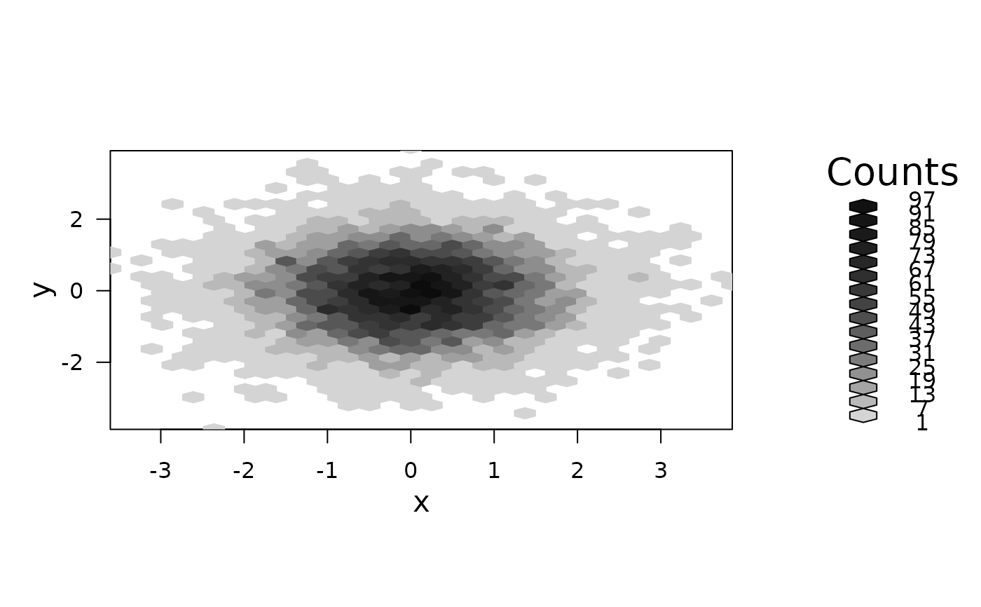 # nested lattice
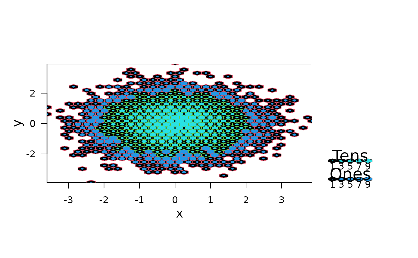
plot(bin, style= "nested.lattice")
# nested lattice
plot(bin, style= "nested.lattice")
 # controlling the colorscheme
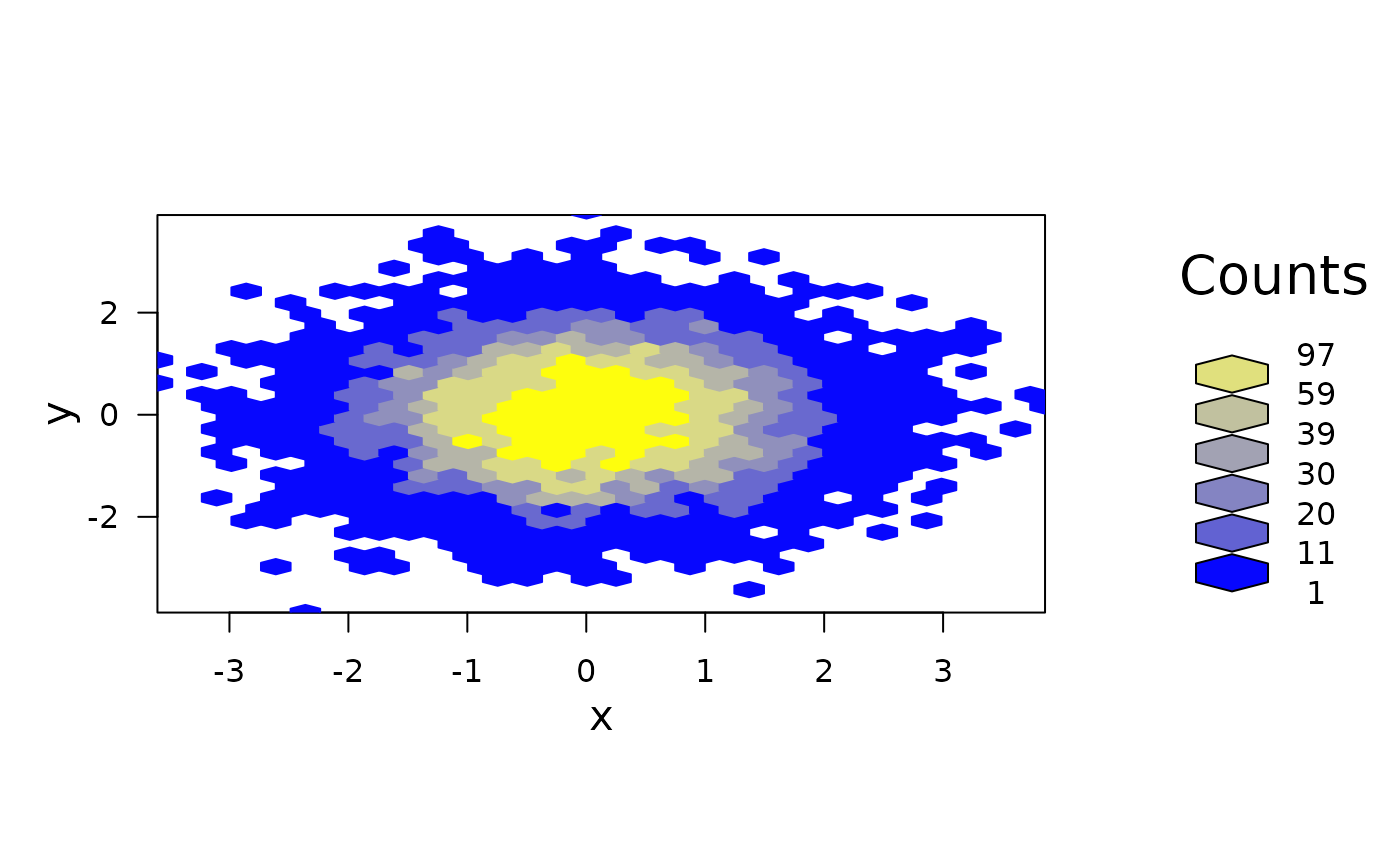
plot(bin, colramp=BTY, colorcut=c(0,.1,.2,.3,.4,.6,1))
# controlling the colorscheme
plot(bin, colramp=BTY, colorcut=c(0,.1,.2,.3,.4,.6,1))
 ## 2) A mixture distribution
x <- c(rnorm(5000),rnorm(5000,4,1.5))
y <- c(rnorm(5000),rnorm(5000,2,3))
bin <- hexbin(x,y)
pens <- cbind(c("#ECE2F0","#A6BDDB","#1C9099"),
c("#FFF7BC","#FEC44F","#D95F0E"))
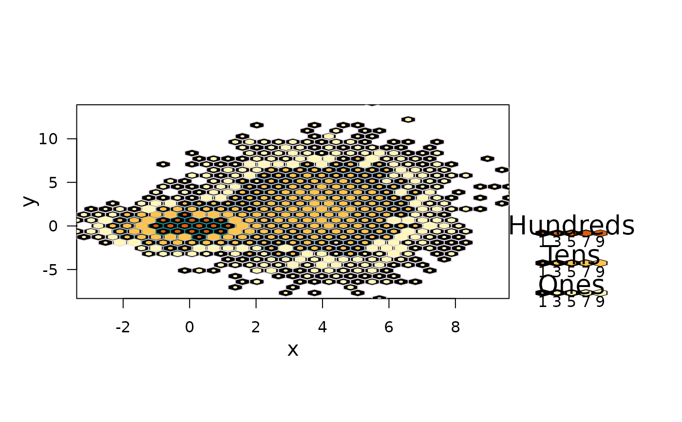
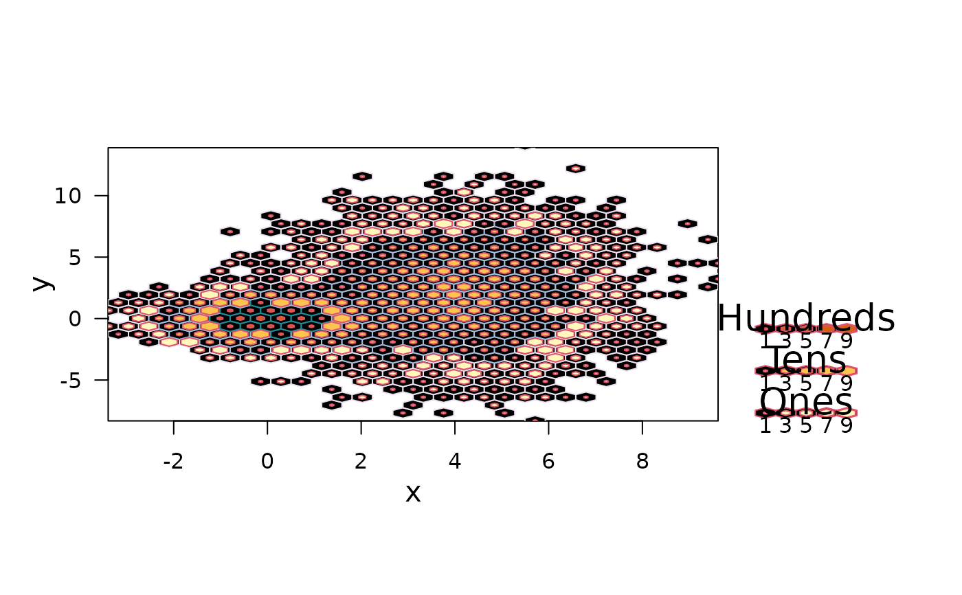
plot(bin, style = "nested.lattice", pen=pens)
## 2) A mixture distribution
x <- c(rnorm(5000),rnorm(5000,4,1.5))
y <- c(rnorm(5000),rnorm(5000,2,3))
bin <- hexbin(x,y)
pens <- cbind(c("#ECE2F0","#A6BDDB","#1C9099"),
c("#FFF7BC","#FEC44F","#D95F0E"))
plot(bin, style = "nested.lattice", pen=pens)
 # now really crazy
plot(bin, style = "nested.lattice", pen=pens,border=2,density=35)
# now really crazy
plot(bin, style = "nested.lattice", pen=pens,border=2,density=35)
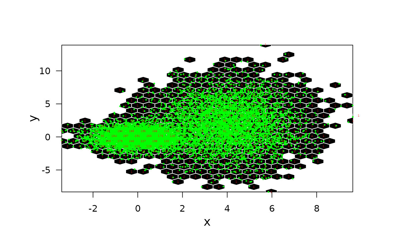
 # lower resolution binning and overplotting with counts
bin <- hexbin(x,y,xbins=25)
P <- plot(bin, style="lattice", legend=FALSE,
minarea=1, maxarea=1, border="white")
##
library("grid")
pushHexport(P$plot.vp)
xy <- hcell2xy(bin)
# to show points rather than counts :
grid.points(x,y,pch=18,gp=gpar(cex=.3,col="green"))
grid.text(as.character(bin@count), xy$x,xy$y,
gp=gpar(cex=0.3, col="red"),default.units="native")
popViewport()
# lower resolution binning and overplotting with counts
bin <- hexbin(x,y,xbins=25)
P <- plot(bin, style="lattice", legend=FALSE,
minarea=1, maxarea=1, border="white")
##
library("grid")
pushHexport(P$plot.vp)
xy <- hcell2xy(bin)
# to show points rather than counts :
grid.points(x,y,pch=18,gp=gpar(cex=.3,col="green"))
grid.text(as.character(bin@count), xy$x,xy$y,
gp=gpar(cex=0.3, col="red"),default.units="native")
popViewport()
 # Be creative, have fun!