Local polynomial fit.
locpoly.RdThis function performs a local polynomial fit of up to order 3 to bivariate data. It returns estimated values of the regression function as well as estimated partial derivatives up to order 3. This access to the partial derivatives was the main intent for writing this code as there already many other local polynomial regression implementations in R.
Arguments
- x
vector of \(x\)-coordinates of data points.
Missing values are not accepted.
- y
vector of \(y\)-coordinates of data points.
Missing values are not accepted.
- z
vector of \(z\)-values at data points.
Missing values are not accepted.
x,y, andzmust be the same length- xo
If
output="grid"(default): sequence of \(x\) locations for rectangular output grid, defaults tonxpoints betweenmin(x)andmax(x).If
output="points": vector of \(x\) locations for output points.- yo
If
output="grid"(default): sequence of \(y\) locations for rectangular output grid, defaults tonypoints betweenmin(y)andmax(y).If
output="points": vector of \(y\) locations for output points. In this case it has to be same length asxo.- input
text, possible values are
"grid"(not yet implemented) and"points"(default).This is used to distinguish between regular and irregular gridded data.
- output
text, possible values are
"grid"(=default) and"points".If
"grid"is choosen thenxoandyoare interpreted as vectors spanning a rectangular grid of points \((xo[i],yo[j])\), \(i=1,...,nx\), \(j=1,...,ny\). This default behaviour matches howakima::interpworks.In the case of
"points"xoandyohave to be of same lenght and are taken as possibly irregular spaced output points \((xo[i],yo[i])\), \(i=1,...,no\) withno=length(xo).nxandnyare ignored in this case.- nx
dimension of output grid in x direction
- ny
dimension of output grid in y direction
- h
bandwidth parameter, between 0 and 1. If a scalar is given it is interpreted as ratio applied to the dataset size to determine a local search neighbourhood, if set to 0 a minimum useful search neighbourhood is choosen (e.g. 10 points for a cubic trend function to determine all 10 parameters).
If a vector of length 2 is given both components are interpreted as ratio of the \(x\)- and \(y\)-range and taken as global bandwidth.
- kernel
Text value, implemented kernels are
uniform,triangle,epanechnikov,biweight,tricube,triweight,cosineandgaussian(default).- solver
Text value, determines used solver in fastLM algorithm used by this code
Possible values are
LLt,QR(default),SVD,EigenandCPivQR(comparefastLm).- degree
Integer value, degree of polynomial trend, maximum allowed value is 3.
- pd
Text value, determines which partial derivative should be returned, possible values are
""(default, the polynomial itself),"x","y","xx","xy","yy","xxx","xxy","xyy","yyy"or"all".
Value
If pd="all":
- x
\(x\) coordinates
- y
\(y\) coordinates
- z
estimates of \(z\)
- zx
estimates of \(dz/dx\)
- zy
estimates of \(dz/dy\)
- zxx
estimates of \(d^2z/dx^2\)
- zxy
estimates of \(d^2z/dxdy\)
- zyy
estimates of \(d^2z/dy^2\)
- zxxx
estimates of \(d^3z/dx^3\)
- zxxy
estimates of \(d^3z/dx^2dy\)
- zxyy
estimates of \(d^3z/dxdy^2\)
- zyyy
estimates of \(d^3z/dy^3\)
If pd!="all" only the elements x, y and the desired
derivative will be returned, e.g. zxy for pd="xy".
References
Douglas Bates, Dirk Eddelbuettel (2013). Fast and Elegant Numerical Linear Algebra Using the RcppEigen Package. Journal of Statistical Software, 52(5), 1-24. URL http://www.jstatsoft.org/v52/i05/.
Author
Albrecht Gebhardt <[email protected]>, Roger Bivand <[email protected]>
Note
Function locpoly of package
KernSmooth performs a similar task for univariate data.
Examples
## choose a kernel
knl <- "gaussian"
## choose global and local bandwidth
bwg <- 0.25 # *100% means: percentage of x- y-range used
bwl <- 0.1 # *100% means: percentage of data set (nearest neighbours) used
## a bivariate polynomial of degree 5:
f <- function(x,y) 0.1+ 0.2*x-0.3*y+0.1*x*y+0.3*x^2*y-0.5*y^2*x+y^3*x^2+0.1*y^5
## degree of model
dg=3
## part 1:
## regular gridded data:
ng<- 11 # x/y size of a square data grid
## build and fill the grid with the theoretical values:
xg<-seq(0,1,length=ng)
yg<-seq(0,1,length=ng)
# xg and yg as matrix matching fg
nx <- length(xg)
ny <- length(yg)
xx <- t(matrix(rep(xg,ny),nx,ny))
yy <- matrix(rep(yg,nx),ny,nx)
fg <- outer(xg,yg,f)
## local polynomial estimate
## global bw:
ttg <- system.time(pdg <- locpoly(xg,yg,fg,
input="grid", pd="all", h=c(bwg,bwg), solver="QR", degree=dg, kernel=knl))
## time used:
ttg
#> user system elapsed
#> 0.067 0.000 0.067
## local bw:
ttl <- system.time(pdl <- locpoly(xg,yg,fg,
input="grid", pd="all", h=bwl, solver="QR", degree=dg, kernel=knl))
## time used:
ttl
#> user system elapsed
#> 0.156 0.001 0.157
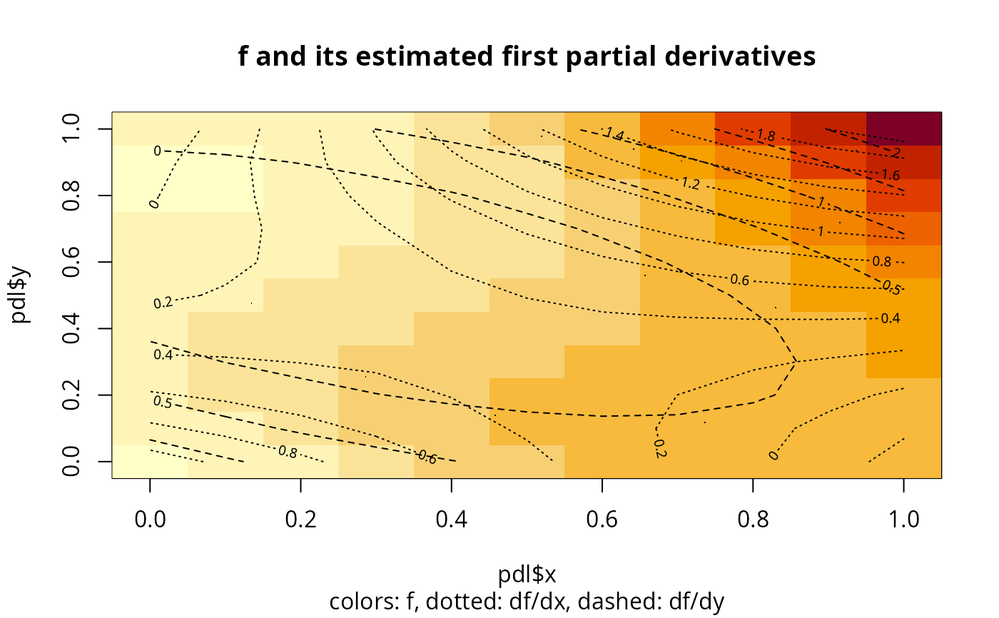
image(pdl$x,pdl$y,pdl$z,main="f and its estimated first partial derivatives",
sub="colors: f, dotted: df/dx, dashed: df/dy")
contour(pdl$x,pdl$y,pdl$zx,add=TRUE,lty="dotted")
contour(pdl$x,pdl$y,pdl$zy,add=TRUE,lty="dashed")
points(xx,yy,pch=".")
 ## part 2:
## irregular data,
## results will not be as good as with the regular 21*21=231 points.
nd<- 121 # size of data set
## random irregular data
oldseed <- set.seed(42)
x<-runif(ng)
y<-runif(ng)
set.seed(oldseed)
z <- f(x,y)
## global bw:
ttg <- system.time(pdg <- interp::locpoly(x,y,z, xg,yg, pd="all",
h=c(bwg,bwg), solver="QR", degree=dg,kernel=knl))
ttg
#> user system elapsed
#> 0.002 0.000 0.003
## local bw:
ttl <- system.time(pdl <- interp::locpoly(x,y,z, xg,yg, pd="all",
h=bwl, solver="QR", degree=dg,kernel=knl))
ttl
#> user system elapsed
#> 0.003 0.000 0.003
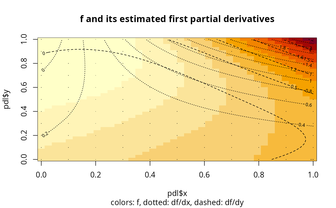
image(pdl$x,pdl$y,pdl$z,main="f and its estimated first partial derivatives",
sub="colors: f, dotted: df/dx, dashed: df/dy")
contour(pdl$x,pdl$y,pdl$zx,add=TRUE,lty="dotted")
contour(pdl$x,pdl$y,pdl$zy,add=TRUE,lty="dashed")
points(x,y,pch=".")
## part 2:
## irregular data,
## results will not be as good as with the regular 21*21=231 points.
nd<- 121 # size of data set
## random irregular data
oldseed <- set.seed(42)
x<-runif(ng)
y<-runif(ng)
set.seed(oldseed)
z <- f(x,y)
## global bw:
ttg <- system.time(pdg <- interp::locpoly(x,y,z, xg,yg, pd="all",
h=c(bwg,bwg), solver="QR", degree=dg,kernel=knl))
ttg
#> user system elapsed
#> 0.002 0.000 0.003
## local bw:
ttl <- system.time(pdl <- interp::locpoly(x,y,z, xg,yg, pd="all",
h=bwl, solver="QR", degree=dg,kernel=knl))
ttl
#> user system elapsed
#> 0.003 0.000 0.003
image(pdl$x,pdl$y,pdl$z,main="f and its estimated first partial derivatives",
sub="colors: f, dotted: df/dx, dashed: df/dy")
contour(pdl$x,pdl$y,pdl$zx,add=TRUE,lty="dotted")
contour(pdl$x,pdl$y,pdl$zy,add=TRUE,lty="dashed")
points(x,y,pch=".")