Normal kernel density estimate for semiparametric EM output

Takes an object of class spEM and returns an object of class density giving the kernel density estimate.

Usage

# S3 method for class 'spEM'
density(x, u=NULL, component=1, block=1, scale=FALSE, ...)

Arguments

x: An object of class npEM such as the output of the npEM or spEMsymloc functions.
u: Vector of points at which the density is to be evaluated
component: Mixture component number; should be an integer from 1 to the number of columns of x$posteriors.
block: Block of repeated measures. Only applicable in repeated measures case, for which x$blockid exists; should be an integer from 1 to max(x$blockid).
scale: Logical: If TRUE, multiply the density values by the corresponding mixing proportions found in x$lambdahat
...: Additional arguments; not used by this method.

Details

The bandwidth is taken to be the same as that used to produce the npEM object, which is given by x$bandwidth.

Value

density.spEM returns a list of type "density". See density for details. In particular, the output of density.spEM may be used directly by functions such as plot or lines.

Examples

set.seed(100)
mu <- matrix(c(0, 15), 2, 3)
sigma <- matrix(c(1, 5), 2, 3)
x <- rmvnormmix(300, lambda = c(.4,.6), mu = mu, sigma = sigma)

d <- spEM(x, mu0 = 2, blockid = rep(1,3), constbw = TRUE) 
#> iteration 1   lambda  0.5767 0.4233 time 0.01 
#> iteration 2   lambda  0.5868 0.4132 time 0.011 
#> iteration 3   lambda  0.5849 0.4151 time 0.01 
#> iteration 4   lambda  0.5849 0.4151 time 0.012 
#> iteration 5   lambda  0.5848 0.4152 time 0.01 
#> iteration 6   lambda  0.5848 0.4152 time 0.011 
#> iteration 7   lambda  0.5848 0.4152 time 0.01 
#> iteration 8   lambda  0.5848 0.4152 time 0.011 
#> lambda  0.5848 0.4152, total time 0.087 s
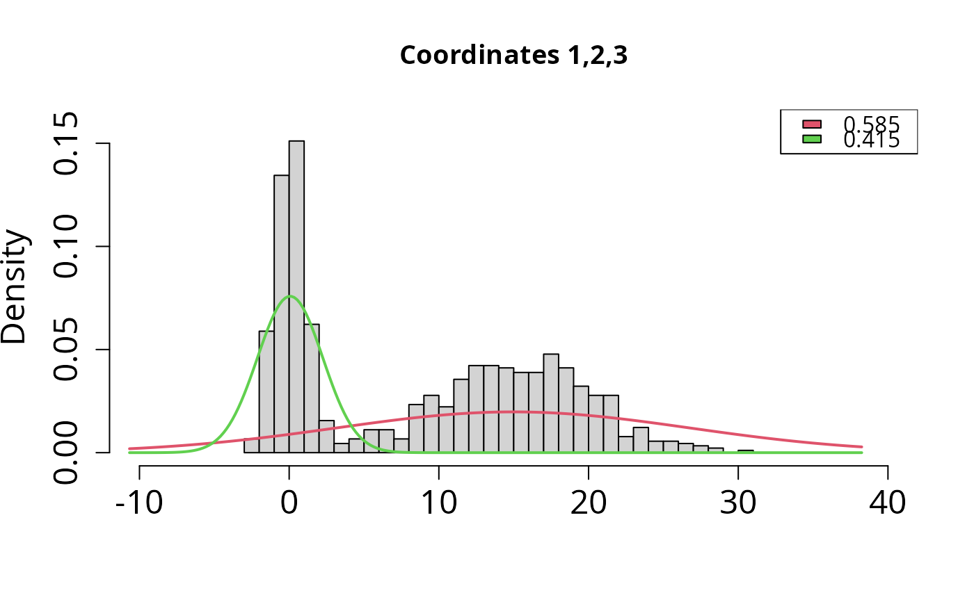
plot(d, xlim=c(-10, 40), ylim = c(0, .16), xlab = "", breaks = 30, 
     cex.lab=1.5, cex.axis=1.5) # plot.spEM calls density.spEM here