EM Algorithm for Mixtures of Regressions with Flare

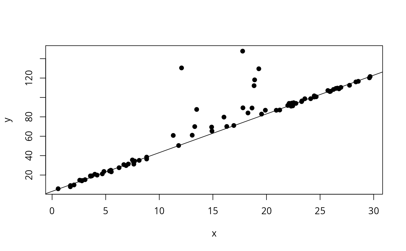
Returns output for 2-component mixture of regressions with flaring using an EM algorithm with one step of Newton-Raphson requiring an adaptive barrier for maximization of the objective function. A mixture of regressions with flare occurs when there appears to be a common regression relationship for the data, but the error terms have a mixture structure of one normal component and one exponential component.

Usage

flaremixEM(y, x, lambda = NULL, beta = NULL, sigma = NULL, 
           alpha = NULL, nu = NULL, epsilon = 1e-04, 
           maxit = 10000, verb = FALSE, restart = 50)

Arguments

y

An n-vector of response values.

x

An n-vector of predictor values. An intercept term will be added by default.

lambda

Initial value of mixing proportions. Entries should sum to 1.

beta

Initial value of beta parameters. Should be a 2x2 matrix where the columns correspond to the component.

sigma

A vector of standard deviations.

alpha

A scalar for the exponential component's rate.

nu

A vector specifying the barrier constants to use. The first barrier constant where the algorithm converges is used.

epsilon

The convergence criterion.

maxit

The maximum number of iterations.

verb

If TRUE, then various updates are printed during each iteration of the algorithm.

restart

The number of times to restart the algorithm in case convergence is not attained. The default is 50.

Value

flaremixEM returns a list of class mixEM with items:

x

The set of predictors (which includes a column of 1's).

y

The response values.

posterior

An nx2 matrix of posterior probabilities for observations.

lambda

The final mixing proportions.

beta

The final regression coefficients.

sigma

The final standard deviations.

alpha

The final exponential rate.

loglik

The final log-likelihood.

all.loglik

A vector of each iteration's log-likelihood.

ft

A character vector giving the name of the function.

See also

regmixEM

Examples

## Simulation output.

set.seed(100)
j=1
while(j == 1){
    x1 <- runif(30, 0, 10)
    x2 <- runif(20, 10, 20)
    x3 <- runif(30, 20, 30)
    y1 <- 3+4*x1+rnorm(30, sd = 1)
    y2 <- 3+4*x2+rexp(20, rate = .05)
    y3 <- 3+4*x3+rnorm(30, sd = 1)
    x <- c(x1, x2, x3)
    y <- c(y1, y2, y3)
    nu <- (1:30)/2

    out <- try(flaremixEM(y, x, beta = c(3, 4), nu = nu,
               lambda = c(.75, .25), sigma = 1), silent = TRUE)
    if(any(class(out) == "try-error")){
        j <- 1
    } else j <- 2
}
#> number of iterations= 14 

out[4:7]
#> $lambda
#> [1] 0.7846493 0.2153507
#> 
#> $beta
#>       [,1]
#>   3.181668
#> x 3.991904
#> 
#> $sigma
#> [1] 1.200692
#> 
#> $alpha
#> [1] 0.0430968
#> 
plot(x, y, pch = 19)
abline(out$beta)