Various Plots Pertaining to Mixture Models

Takes an object of class mixEM and returns various graphical output for select mixture models.

Usage

# S3 method for class 'mixEM'
plot(x, whichplots = 1, 
     loglik = 1 %in% whichplots,
     density = 2 %in% whichplots,
     xlab1="Iteration", ylab1="Log-Likelihood",
     main1="Observed Data Log-Likelihood", col1=1, lwd1=2,
     xlab2=NULL, ylab2=NULL, main2=NULL, col2=NULL, 
     lwd2=2, alpha = 0.05, marginal = FALSE, ...)

Arguments

x

An object of class mixEM.

whichplots

vector telling which plots to produce: 1 = loglikelihood plot, 2 = density plot. Irrelevant if loglik and density are specified.

loglik

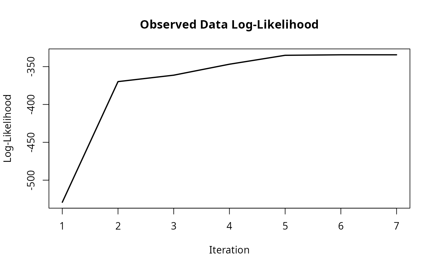
If TRUE, a plot of the log-likelihood versus the EM iterations is given.

density

Graphics pertaining to certain mixture models. The details are given below.

xlab1, ylab1, main1, col1, lwd1

Graphical parameters xlab, ..., lwd to be passed to the loglikelihood plot. Trying to change these parameters using xlab, ..., lwd will result in an error, but all other graphical parameters are passed directly to the plotting functions via ...

xlab2, ylab2, main2, col2, lwd2

Same as xlab1 etc. but for the density plot

alpha

A vector of significance levels when constructing confidence ellipses and confidence bands for the mixture of multivariate normals and mixture of regressions cases, respectively. The default is 0.05.

marginal

For the mixture of bivariate normals, should optional marginal histograms be included?

...

Graphical parameters passed to plot command.

Value

plot.mixEM returns a plot of the log-likelihood versus the EM iterations by default for all objects of class mixEM. In addition, other plots may be produced for the following k-component mixture model functions:

normalmixEM

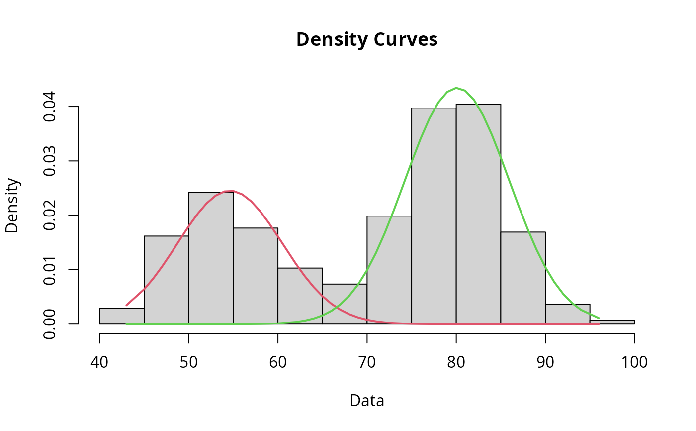
A histogram of the raw data is produced along with k density curves determined by normalmixEM.

repnormmixEM

A histogram of the raw data produced in a similar manner as for normalmixEM.

mvnormalmixEM

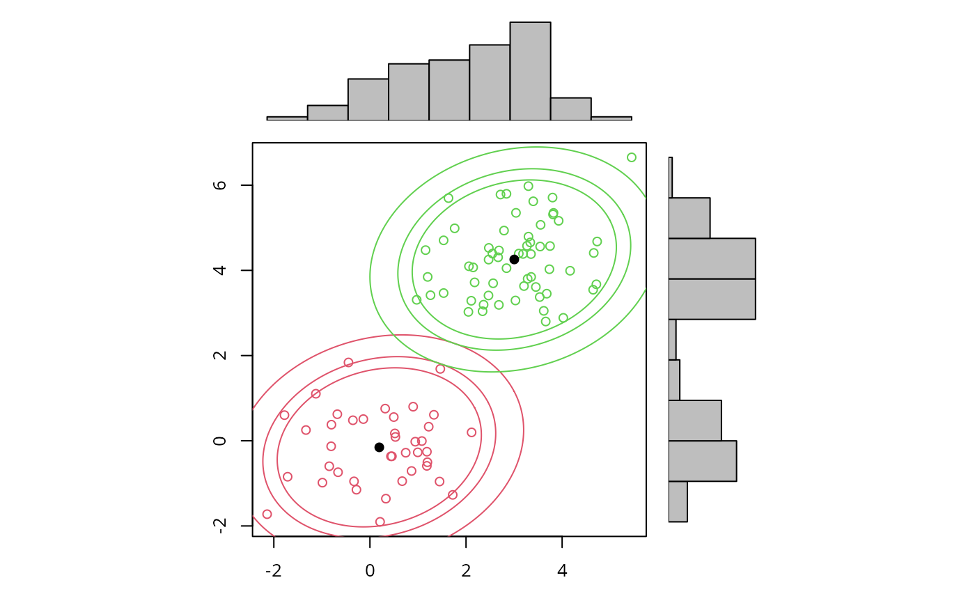
A 2-dimensional plot with each point color-coded to denote its most probable component membership. In addition, the estimated component means are plotted along with (1 - alpha)% bivariate normal density contours. These ellipses are constructed by assigning each value to their component of most probable membership and then using normal theory. Optional marginal histograms may also be produced.

regmixEM

A plot of the response versus the predictor with each point color-coded to denote its most probable component membership. In addition, the estimated component regression lines are plotted along with (1 - alpha)% Working-Hotelling confidence bands. These bands are constructed by assigning each value to their component of most probable membership and then performing least squares estimation.

logisregmixEM

A plot of the binary response versus the predictor with each point color-coded to denote its most probable compopnent membership. In addition, the estimate component logistic regression lines are plotted.

regmixEM.mixed

Provides a 2x2 matrix of plots summarizing the posterior slope and posterior intercept terms from a mixture of random effects regression. See post.beta for a more detailed description.

See also

post.beta

Examples

##Analyzing the Old Faithful geyser data with a 2-component mixture of normals.

data(faithful)
attach(faithful)
#> The following objects are masked from faithful (pos = 3):
#> 
#>     eruptions, waiting
#> The following objects are masked from faithful (pos = 4):
#> 
#>     eruptions, waiting
set.seed(100)
out <- normalmixEM(waiting, arbvar = FALSE, verb = TRUE,
                   epsilon = 1e-04)
#> iteration = 1  log-lik diff = 90.60371  log-lik = -1077.998 
#>              [,1]       [,2]
#> lambda  0.2811183  0.7188817
#> mu     53.4667182 77.7131826
#> sigma  10.2937749 10.2937749
#> iteration = 2  log-lik diff = 18.87546  log-lik = -1059.123 
#>              [,1]       [,2]
#> lambda  0.2952884  0.7047116
#> mu     54.3806159 77.8177824
#> sigma   8.3721214  8.3721214
#> iteration = 3  log-lik diff = 16.66864  log-lik = -1042.454 
#>              [,1]       [,2]
#> lambda  0.3247154  0.6752846
#> mu     54.1253887 78.9618363
#> sigma   7.0561343  7.0561343
#> iteration = 4  log-lik diff = 7.242952  log-lik = -1035.211 
#>             [,1]      [,2]
#> lambda  0.345328  0.654672
#> mu     54.279887 79.662327
#> sigma   6.230516  6.230516
#> iteration = 5  log-lik diff = 1.101903  log-lik = -1034.109 
#>              [,1]       [,2]
#> lambda  0.3553761  0.6446239
#> mu     54.4702326 79.9530407
#> sigma   5.9540013  5.9540013
#> iteration = 6  log-lik diff = 0.09855678  log-lik = -1034.011 
#>              [,1]       [,2]
#> lambda  0.3591139  0.6408861
#> mu     54.5638934 80.0491791
#> sigma   5.8881061  5.8881061
#> iteration = 7  log-lik diff = 0.008087694  log-lik = -1034.002 
#>             [,1]      [,2]
#> lambda  0.360324  0.639676
#> mu     54.597872 80.078250
#> sigma   5.873570  5.873570
#> iteration = 8  log-lik diff = 0.0006757765  log-lik = -1034.002 
#>              [,1]       [,2]
#> lambda  0.3606935  0.6393065
#> mu     54.6088420 80.0867894
#> sigma   5.8702283  5.8702283
#> iteration = 9  log-lik diff = 5.723897e-05  log-lik = -1034.002 
#>              [,1]       [,2]
#> lambda  0.3608036  0.6391964
#> mu     54.6122032 80.0892796
#> sigma   5.8693982  5.8693982
#> number of iterations= 9 
plot(out, density = TRUE, w = 1.1)


##Fitting randomly generated data with a 2-component location mixture of bivariate normals.

x.1 <- rmvnorm(40, c(0, 0))
x.2 <- rmvnorm(60, c(3, 4))
X.1 <- rbind(x.1, x.2)

out.1 <- mvnormalmixEM(X.1, arbvar = FALSE, verb = TRUE,
                       epsilon = 1e-03)
#> iteration= 1 diff= 159.3998 log-likelihood -369.8147 
#> iteration= 2 diff= 8.502903 log-likelihood -361.3118 
#> iteration= 3 diff= 14.48476 log-likelihood -346.827 
#> iteration= 4 diff= 11.78277 log-likelihood -335.0443 
#> iteration= 5 diff= 0.6490807 log-likelihood -334.3952 
#> iteration= 6 diff= 0.0003704159 log-likelihood -334.3948 
#> number of iterations= 6 
plot(out.1, density = TRUE, alpha = c(0.01, 0.05, 0.10), 
     marginal = TRUE)