semiparametric EM-like algorithm for univariate mixture in False Discovery Rate (FDR) estimation
spEMsymlocN01.RdReturn semiparametric EM-like algorithm output for a 2-components
mixture model with one component set to Normal(0,1), and the other component
being a unspecified but symmetric density with a location parameter.
This model is tailored to
FDR estimation on probit transform (qnorm) of p-values arising from multiple testing.
Usage
spEMsymlocN01(x, mu0 = 2, bw = bw.nrd0(x), h=bw, eps = 1e-8,
              maxiter = 100, verbose = FALSE, plotf = FALSE)
Arguments
- x
A vector of length n consisting of the data, probit transform of pvalues, preferably sorted.
- mu0
Starting value of vector of component means. If not set then the initial value is randomly generated by a
kmeansof the data in two bins. Since component 1 is theoretically normal(0,1),mu[1]must be 0 andmu[2]some negative value (see details).- bw
Bandwidth for weighted kernel density estimation.
- h
Alternative way to specify the bandwidth, to provide backward compatibility.
- eps
Tolerance limit for declaring algorithm convergence. Convergence is declared before
maxiteriterations whenever the maximum change in any coordinate of thelambda(mixing proportion estimates) andmu(mean of the semiparametric component) vector does not exceedeps- maxiter
The maximum number of iterations allowed; convergence may be declared before
maxiteriterations (seeepsabove).- verbose
If TRUE, print updates for every iteration of the algorithm as it runs.
- plotf
If TRUE, plots successive updates of the nonparametric density estimate over iterations. Mostly for testing purpose.
Details
This algorithm is a specific version of semiparametric EM-like algorithm
similar in spirit to spEMsymloc, but specialized for FDR estimation on
probit transform (qnorm) of p-values in multiple testing framework.
In this model, component 1 corresponds to the individuals under the null hypothesis,
i.e. theoretically normal(0,1) distributed, whereas component 2 corresponds to individuals in the
alternative hypothesis, with typically very small p-values and consequently
negative values for probit(p) data. This model only assumes
that these individuals come from an unspecified but symmetric density with a location parameter,
as in Bordes and Vandekerkhove (2010) and Chauveau et al. (2014).
Value
spEMsymlocN01 returns a list of class spEMN01 with the following items:
- data
The raw data (an \(n\times r\) matrix).
- posteriors
An \(n\times 2\) matrix of posterior probabilities for observations. This can be used in, e.g.,
plotFDRto plot False Discovery Rate estimates.- bandwidth
Same as the
bwinput argument, returned because this information is needed by any method that produces density estimates from the output.- lambda
The sequence of mixing proportions over iterations.
- lambdahat
The final estimate for mixing proportions.
- mu
the sequence of second component mean over iterations.
- muhat
the final estimate of second component mean.
- symmetric
Flag indicating that the kernel density estimate is using a symmetry assumption.
References
Bordes, L. and Vandekerkhove, P. (2010). Semiparametric two-component mixture model with a known component: an asymptotically normal estimator. Mathematical Methods of Statistics, 19(1):22-41
Chauveau, D., Saby, N., Orton, T. G., Lemercier B., Walter, C. and Arrouys, D. (2014) Large-scale simultaneous hypothesis testing in monitoring carbon content from french soil database: A semi-parametric mixture approach. Geoderma 219-220 (2014): 117-124.
Examples
## Probit transform of p-values
## from a Beta-Uniform mixture model
## comparion of parametric and semiparametric EM fit
## Note: in actual situations n=thousands
set.seed(50)
n=300 # nb of multiple tests
m=2 # 2 mixture components
a=c(1,0.1); b=c(1,1); lambda=c(0.6,0.4) # parameters
z=sample(1:m, n, rep=TRUE, prob = lambda)
p <- rbeta(n, shape1 = a[z], shape2 = b[z]) # p-values
o <- order(p)
cpd <- cbind(z,p)[o,] # sorted complete data, z=1 if H0, 2 if H1
p <- cpd[,2] # sorted p-values
y <- qnorm(p) # probit transform of the pvalues
# gaussian EM fit with component 1 constrained to N(0,1)
s1 <- normalmixEM(y, mu=c(0,-4),
mean.constr = c(0,NA), sd.constr = c(1,NA))
#> number of iterations= 49
s2 <- spEMsymlocN01(y, mu0 = c(0,-3)) # spEM with N(0,1) fit
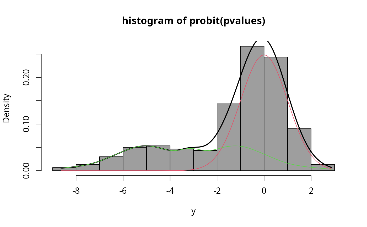
hist(y, freq = FALSE, col = 8, main = "histogram of probit(pvalues)")
plot(s2, add.plot = TRUE, lwd = 2)
 # Exemples of plot capabilities
# Note: posteriors must be ordered by p for plot.FDR
# plotFDR(s1$post) # when true complete data not observed
# plotFDR(s1$post, s2$post) # comparing 2 strategies
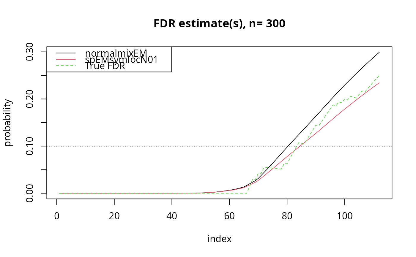
plotFDR(s1$post, s2$post, lg1 = "normalmixEM", lg2 = "spEMsymlocN01",
complete.data = cpd) # with true FDR computed from z
# Exemples of plot capabilities
# Note: posteriors must be ordered by p for plot.FDR
# plotFDR(s1$post) # when true complete data not observed
# plotFDR(s1$post, s2$post) # comparing 2 strategies
plotFDR(s1$post, s2$post, lg1 = "normalmixEM", lg2 = "spEMsymlocN01",
complete.data = cpd) # with true FDR computed from z