EM-like Algorithm for Semiparametric Mixtures of Regressions
spregmix.RdReturns parameter estimates for finite mixtures of linear regressions with unspecified error structure. Based on Hunter and Young (2012).
Arguments
- lmformula
Formula for a linear model, in the same format used by
lm. Additional parameters may be passed tolmvia the...argument.- bw
Initial bandwidth value. If NULL, this will be chosen automatically by the algorithm.
- constbw
Logical: If TRUE, the bandwidth is held constant throughout the algorithm; if FALSE, it adapts at each iteration according to the rules given in Hunter and Young (2012).
- bwmult
Whenever it is updated automatically, the bandwidth is equal to
bwmultdivided by the fifth root of \(n\) times the smaller of s and IQR/1.34, where s and IQR are estimates of the standard deviation and interquartile range of the residuals, as explained in Hunter and Young (2012). The value of 0.9 gives the rule of Silverman (1986) and the value of 1.06 gives the rule of Scott (1992). Larger values lead to greater smoothing, whereas smaller values lead to less smoothing.- z.hat
Initial nxm matrix of posterior probabilities. If NULL, this is initialized randomly. As long as a parametric estimation method like least squares is used to estimate
betain each M-step, thez.hatvalues are the only values necessary to begin the EM iterations.- symm
Logical: If TRUE, the error density is assumed symmetric about zero. If FALSE, it is not. WARNING: If FALSE, the intercept parameter is not uniquely identifiable if it is included in the linear model.
- betamethod
Method of calculating beta coefficients in the M-step. Current possible values are "LS" for least-squares; "L1" for least absolute deviation; "NP" for fully nonparametric; and "transition" for a transition from least squares to fully nonparametric. If something other than these four possibilities is used, then "NP" is assumed. For details of these methods, see Hunter and Young (2012).
- m
Number of components in the mixture.
- epsilon
Convergence is declared if the largest change in any lambda or beta coordinate is smaller than
epsilon.- maxit
The maximum number of iterations; if convergence is never declared based on comparison with
epsilon, then the algorithm stops aftermaxititerations.- verbose
Logical: If TRUE, then various updates are printed during each iteration of the algorithm.
- ...
Additional parameters passed to the
model.frameandmodel.matrixfunctions, which are used to obtain the response and predictor of the regression.
Value
regmixEM returns a list of class npEM with items:
- x
The set of predictors (which includes a column of 1's if
addintercept= TRUE).- y
The response values.
- lambda
The mixing proportions for every iteration in the form of a matrix with m columns and (#iterations) rows
- beta
The final regression coefficients.
- posterior
An nxm matrix of posterior probabilities for observations.
- np.stdev
Nonparametric estimate of the standard deviation, as given in Hunter and Young (2012)
- bandwidth
Final value of the bandwidth
- density.x
Points at which the error density is estimated
- density.y
Values of the error density at the points
density.x- symmetric
Logical: Was the error density assumed symmetric?
- loglik
A quantity similar to a log-likelihood, computed just like a standard loglikelihood would be, conditional on the component density functions being equal to the final density estimates.
- ft
A character vector giving the name of the function.
References
Hunter, D. R. and Young, D. S. (2012) Semi-parametric Mixtures of Regressions, Journal of Nonparametric Statistics 24(1): 19-38.
Scott, D. W. (1992) Multivariate Density Estimation, John Wiley & Sons Inc., New York.
Silverman, B. W. (1986). Density Estimation for Statistics and Data Analysis, Chapman & Hall, London.
Examples
data(tonedata)
## By default, the bandwidth will adapt and the error density is assumed symmetric
set.seed(100)
a=spregmix(tuned~stretchratio, bw=.2, data=tonedata, verb=TRUE)
#> iteration 1 lambda 0.4919 0.5081 bandwidth 0.064 time 0.002
#> iteration 2 lambda 0.4984 0.5016 bandwidth 0.059 time 0.001
#> iteration 3 lambda 0.5114 0.4886 bandwidth 0.055 time 0.001
#> iteration 4 lambda 0.5335 0.4665 bandwidth 0.044 time 0.001
#> iteration 5 lambda 0.5722 0.4278 bandwidth 0.034 time 0.001
#> iteration 6 lambda 0.6279 0.3721 bandwidth 0.025 time 0.001
#> iteration 7 lambda 0.6572 0.3428 bandwidth 0.02 time 0.002
#> iteration 8 lambda 0.6657 0.3343 bandwidth 0.017 time 0.001
#> iteration 9 lambda 0.665 0.335 bandwidth 0.018 time 0.002
#> iteration 10 lambda 0.6669 0.3331 bandwidth 0.019 time 0.002
#> iteration 11 lambda 0.6703 0.3297 bandwidth 0.02 time 0.001
#> iteration 12 lambda 0.6733 0.3267 bandwidth 0.02 time 0.002
#> iteration 13 lambda 0.6754 0.3246 bandwidth 0.02 time 0.001
#> iteration 14 lambda 0.6765 0.3235 bandwidth 0.02 time 0.001
#> iteration 15 lambda 0.677 0.323 bandwidth 0.02 time 0.002
#> iteration 16 lambda 0.6771 0.3229 bandwidth 0.021 time 0.001
#> iteration 17 lambda 0.6772 0.3228 bandwidth 0.021 time 0.001
#> iteration 18 lambda 0.6772 0.3228 bandwidth 0.021 time 0.001
#> iteration 19 lambda 0.6771 0.3229 bandwidth 0.021 time 0.002
#> iteration 20 lambda 0.6769 0.3231 bandwidth 0.021 time 0.001
#> iteration 21 lambda 0.6768 0.3232 bandwidth 0.021 time 0.002
#> iteration 22 lambda 0.6766 0.3234 bandwidth 0.021 time 0.001
#> iteration 23 lambda 0.6766 0.3234 bandwidth 0.021 time 0.002
#> lambda 0.6766 0.3234, total time 0.034 s
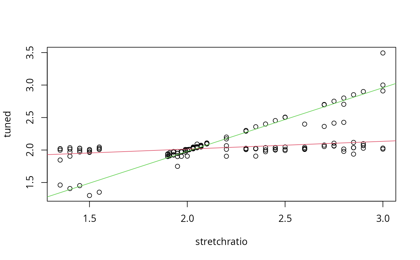
## Look at the sp mixreg solution:
plot(tonedata)
abline(a=a$beta[1,1],b=a$beta[2,1], col=2)
abline(a=a$beta[1,2],b=a$beta[2,2], col=3)
 ## Look at the nonparametric KD-based estimate of the error density,
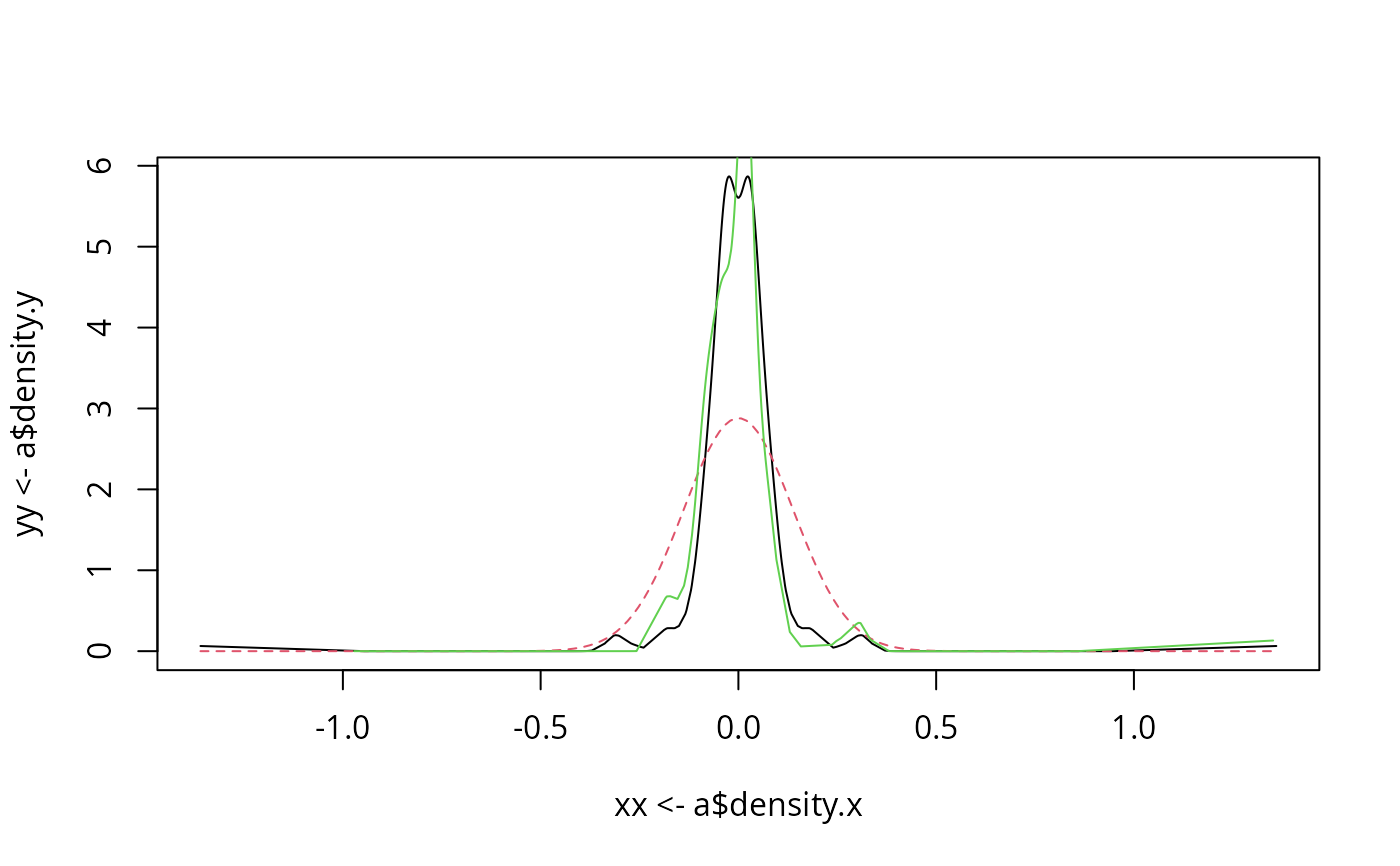
## constrained to be zero-symmetric:
plot(xx<-a$density.x, yy<-a$density.y, type="l")
## Compare to a normal density with mean 0 and NP-estimated stdev:
z <- seq(min(xx), max(xx), len=200)
lines(z, dnorm(z, sd=sqrt((a$np.stdev)^2+a$bandwidth^2)), col=2, lty=2)
# Add bandwidth^2 to variance estimate to get estimated var of KDE
## Now add the sp mixreg estimate without assuming symmetric errors:
b=spregmix(tuned~stretchratio, bw=.2, , symm=FALSE, data=tonedata, verb=TRUE)
#> iteration 1 lambda 0.4924 0.5076 bandwidth 0.066 time 0.002
#> iteration 2 lambda 0.4918 0.5082 bandwidth 0.064 time 0.001
#> iteration 3 lambda 0.4917 0.5083 bandwidth 0.064 time 0.001
#> iteration 4 lambda 0.4921 0.5079 bandwidth 0.065 time 0.001
#> iteration 5 lambda 0.4932 0.5068 bandwidth 0.063 time 0.001
#> iteration 6 lambda 0.4952 0.5048 bandwidth 0.064 time 0.001
#> iteration 7 lambda 0.4985 0.5015 bandwidth 0.064 time 0.001
#> iteration 8 lambda 0.5038 0.4962 bandwidth 0.064 time 0.001
#> iteration 9 lambda 0.5119 0.4881 bandwidth 0.061 time 0.001
#> iteration 10 lambda 0.5245 0.4755 bandwidth 0.06 time 0.002
#> iteration 11 lambda 0.5437 0.4563 bandwidth 0.054 time 0.001
#> iteration 12 lambda 0.5718 0.4282 bandwidth 0.044 time 0.001
#> iteration 13 lambda 0.6099 0.3901 bandwidth 0.036 time 0.001
#> iteration 14 lambda 0.6526 0.3474 bandwidth 0.027 time 0.001
#> iteration 15 lambda 0.6686 0.3314 bandwidth 0.021 time 0.002
#> iteration 16 lambda 0.6748 0.3252 bandwidth 0.02 time 0.001
#> iteration 17 lambda 0.6725 0.3275 bandwidth 0.02 time 0.002
#> iteration 18 lambda 0.6701 0.3299 bandwidth 0.02 time 0.001
#> iteration 19 lambda 0.6678 0.3322 bandwidth 0.02 time 0.002
#> iteration 20 lambda 0.6658 0.3342 bandwidth 0.02 time 0.001
#> iteration 21 lambda 0.6643 0.3357 bandwidth 0.02 time 0.002
#> iteration 22 lambda 0.6642 0.3358 bandwidth 0.02 time 0.001
#> iteration 23 lambda 0.6648 0.3352 bandwidth 0.02 time 0.001
#> iteration 24 lambda 0.6657 0.3343 bandwidth 0.02 time 0.001
#> iteration 25 lambda 0.6664 0.3336 bandwidth 0.02 time 0.002
#> iteration 26 lambda 0.6669 0.3331 bandwidth 0.02 time 0.001
#> iteration 27 lambda 0.6674 0.3326 bandwidth 0.02 time 0.002
#> iteration 28 lambda 0.6679 0.3321 bandwidth 0.02 time 0.001
#> iteration 29 lambda 0.6682 0.3318 bandwidth 0.02 time 0.002
#> iteration 30 lambda 0.6685 0.3315 bandwidth 0.02 time 0.001
#> iteration 31 lambda 0.6687 0.3313 bandwidth 0.02 time 0.002
#> iteration 32 lambda 0.6688 0.3312 bandwidth 0.02 time 0.002
#> iteration 33 lambda 0.6689 0.3311 bandwidth 0.02 time 0.001
#> iteration 34 lambda 0.669 0.331 bandwidth 0.02 time 0.001
#> lambda 0.669 0.331, total time 0.046 s
lines(b$density.x, b$density.y, col=3)
## Look at the nonparametric KD-based estimate of the error density,
## constrained to be zero-symmetric:
plot(xx<-a$density.x, yy<-a$density.y, type="l")
## Compare to a normal density with mean 0 and NP-estimated stdev:
z <- seq(min(xx), max(xx), len=200)
lines(z, dnorm(z, sd=sqrt((a$np.stdev)^2+a$bandwidth^2)), col=2, lty=2)
# Add bandwidth^2 to variance estimate to get estimated var of KDE
## Now add the sp mixreg estimate without assuming symmetric errors:
b=spregmix(tuned~stretchratio, bw=.2, , symm=FALSE, data=tonedata, verb=TRUE)
#> iteration 1 lambda 0.4924 0.5076 bandwidth 0.066 time 0.002
#> iteration 2 lambda 0.4918 0.5082 bandwidth 0.064 time 0.001
#> iteration 3 lambda 0.4917 0.5083 bandwidth 0.064 time 0.001
#> iteration 4 lambda 0.4921 0.5079 bandwidth 0.065 time 0.001
#> iteration 5 lambda 0.4932 0.5068 bandwidth 0.063 time 0.001
#> iteration 6 lambda 0.4952 0.5048 bandwidth 0.064 time 0.001
#> iteration 7 lambda 0.4985 0.5015 bandwidth 0.064 time 0.001
#> iteration 8 lambda 0.5038 0.4962 bandwidth 0.064 time 0.001
#> iteration 9 lambda 0.5119 0.4881 bandwidth 0.061 time 0.001
#> iteration 10 lambda 0.5245 0.4755 bandwidth 0.06 time 0.002
#> iteration 11 lambda 0.5437 0.4563 bandwidth 0.054 time 0.001
#> iteration 12 lambda 0.5718 0.4282 bandwidth 0.044 time 0.001
#> iteration 13 lambda 0.6099 0.3901 bandwidth 0.036 time 0.001
#> iteration 14 lambda 0.6526 0.3474 bandwidth 0.027 time 0.001
#> iteration 15 lambda 0.6686 0.3314 bandwidth 0.021 time 0.002
#> iteration 16 lambda 0.6748 0.3252 bandwidth 0.02 time 0.001
#> iteration 17 lambda 0.6725 0.3275 bandwidth 0.02 time 0.002
#> iteration 18 lambda 0.6701 0.3299 bandwidth 0.02 time 0.001
#> iteration 19 lambda 0.6678 0.3322 bandwidth 0.02 time 0.002
#> iteration 20 lambda 0.6658 0.3342 bandwidth 0.02 time 0.001
#> iteration 21 lambda 0.6643 0.3357 bandwidth 0.02 time 0.002
#> iteration 22 lambda 0.6642 0.3358 bandwidth 0.02 time 0.001
#> iteration 23 lambda 0.6648 0.3352 bandwidth 0.02 time 0.001
#> iteration 24 lambda 0.6657 0.3343 bandwidth 0.02 time 0.001
#> iteration 25 lambda 0.6664 0.3336 bandwidth 0.02 time 0.002
#> iteration 26 lambda 0.6669 0.3331 bandwidth 0.02 time 0.001
#> iteration 27 lambda 0.6674 0.3326 bandwidth 0.02 time 0.002
#> iteration 28 lambda 0.6679 0.3321 bandwidth 0.02 time 0.001
#> iteration 29 lambda 0.6682 0.3318 bandwidth 0.02 time 0.002
#> iteration 30 lambda 0.6685 0.3315 bandwidth 0.02 time 0.001
#> iteration 31 lambda 0.6687 0.3313 bandwidth 0.02 time 0.002
#> iteration 32 lambda 0.6688 0.3312 bandwidth 0.02 time 0.002
#> iteration 33 lambda 0.6689 0.3311 bandwidth 0.02 time 0.001
#> iteration 34 lambda 0.669 0.331 bandwidth 0.02 time 0.001
#> lambda 0.669 0.331, total time 0.046 s
lines(b$density.x, b$density.y, col=3)