Special EM Algorithm for three-component tau equivalence model

Return ECM algorithm output for a specific case of a three-component tau equivalence model

Usage

tauequivnormalmixEM (x, lambda = NULL, mu = NULL, sigma = NULL, k = 3, 
          mean.constr = NULL, sd.constr = NULL, gparam = NULL,
          epsilon = 1e-08, maxit = 10000, maxrestarts=20, 
          verb = FALSE, fast=FALSE, ECM = TRUE,
          arbmean = TRUE, arbvar = TRUE)

Details

The tauequivnormalmixEM function is merely a wrapper for the normalmixMMlc function. # This is the standard EM algorithm for normal mixtures that maximizes # the conditional expected complete-data # log-likelihood at each M-step of the algorithm. # If desired, the # EM algorithm may be replaced by an ECM algorithm (see ECM argument) # that alternates between maximizing with respect to the mu # and lambda while holding sigma fixed, and maximizing with # respect to sigma and lambda while holding mu # fixed. In the case where arbmean is FALSE # and arbvar is TRUE, there is no closed-form EM algorithm, # so the ECM option is forced in this case.

Arguments

x: A vector of length n consisting of the data, passed directly to normalmixMMlc.
lambda: Initial value of mixing proportions, passed directly to normalmixMMlc. Automatically repeated as necessary to produce a vector of length k, then normalized to sum to 1. If NULL, then lambda is random from a uniform Dirichlet distribution (i.e., its entries are uniform random and then it is normalized to sum to 1).
mu: Starting value of vector of component means for algorithm, passed directly to normalmixMMlc. If non-NULL and a vector, k is set to length(mu). If NULL, then the initial value is randomly generated from a normal distribution with center(s) determined by binning the data.
sigma: Starting value of vector of component standard deviations for algorithm, passed directly to normalmixMMlc. Obsolete for linear constraint on the inverse variances, use gparam instead to specify a starting value. Note: This needs more precision
k: Number of components, passed directly to normalmixMMlc. Initial value ignored unless mu and sigma are both NULL. Also, initial value is ignored if mean.constr is NULL, since in that case we presume k=3.
mean.constr: If non-NULL, this parameter is passed directly to normalmixMMlc and both mean.lincstr and var.lincstr are passed as NULL to normalmixMMlc. If NULL, then it is assumed that k=3 and the means must take the form \(\alpha\), \(\alpha-\delta\), and \(\alpha+\delta\) for unknown parameters \(\alpha\) and \(\delta\). Furthermore, the reciprocal variances are assumed to be \(\gamma_1+\gamma_2\), \(\gamma_1\), and \(\gamma_1\) for unknown positive parameters \(\gamma_1\) and \(\gamma_2\). These constraints are passed to the normalmixMMlc function using the mean.lincstr and var.lincstr arguments as shown in the examples for the normalmixMMlc help file.
sd.constr: Deprecated.
gparam: This argument is passed directly to normalmixMMlc.
epsilon: The convergence criterion. Convergence is declared when the change in the observed data log-likelihood increases by less than epsilon.
maxit: The maximum number of iterations.
maxrestarts: The maximum number of restarts allowed in case of a problem with the particular starting values chosen due to one of the variance estimates getting too small (each restart uses randomly chosen starting values). It is well-known that when each component of a normal mixture may have its own mean and variance, the likelihood has no maximizer; in such cases, we hope to find a "nice" local maximum with this algorithm instead, but occasionally the algorithm finds a "not nice" solution and one of the variances goes to zero, driving the likelihood to infinity.
verb: If TRUE, then various updates are printed during each iteration of the algorithm.
fast: If TRUE and k==2 and arbmean==TRUE, then use normalmixEM2comp, which is a much faster version of the EM algorithm for this case. This version is less protected against certain kinds of underflow that can cause numerical problems and it does not permit any restarts. If k>2, fast is ignored.
ECM: logical: Should this algorithm be an ECM algorithm in the sense of Meng and Rubin (1993)? If FALSE, the algorithm is a true EM algorithm; if TRUE, then every half-iteration alternately updates the means conditional on the variances or the variances conditional on the means, with an extra E-step in between these updates. For tauequivnormalmixEM, it must be TRUE.
arbmean: Deprecated.
arbvar: Deprecated.

Value

normalmixEM returns a list of class mixEM with items:

x: The raw data.
lambda: The final mixing proportions.
mu: The final mean parameters.
sigma: The final standard deviation(s)
scale: Scale factor for the component standard deviations, if applicable.
loglik: The final log-likelihood.
posterior: An nxk matrix of posterior probabilities for observations.
all.loglik: A vector of each iteration's log-likelihood. This vector includes both the initial and the final values; thus, the number of iterations is one less than its length.
restarts: The number of times the algorithm restarted due to unacceptable choice of initial values.
ft: A character vector giving the name of the function.

References

Thomas, H., Lohaus, A., and Domsch, H. (2011) Stable Unstable Reliability Theory, British Journal of Mathematical and Statistical Psychology 65(2): 201-221.
Meng, X.-L. and Rubin, D. B. (1993) Maximum Likelihood Estimation Via the ECM Algorithm: A General Framework, Biometrika 80(2): 267-278.

Examples

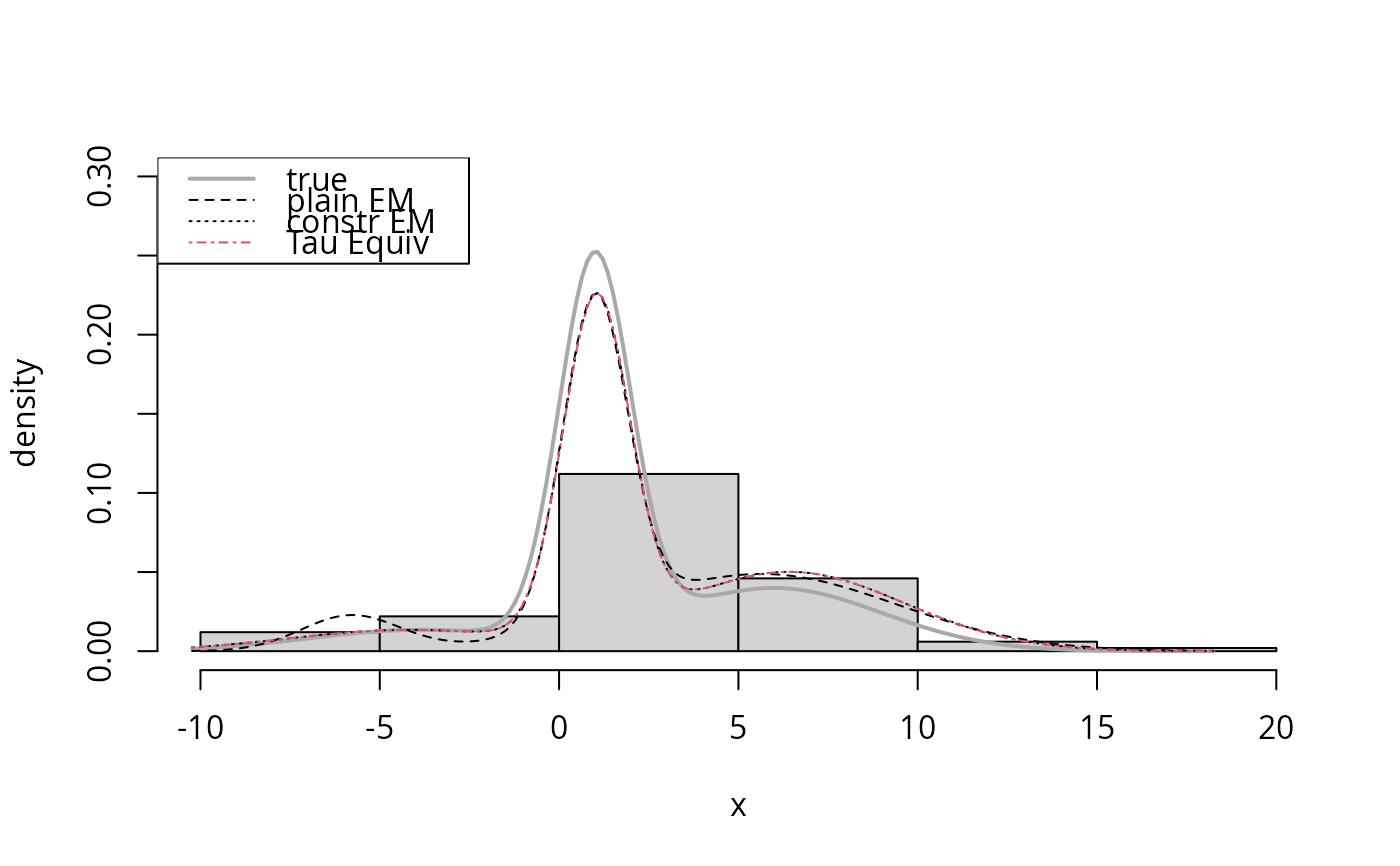
## Analyzing synthetic data as in the tau equivalent model  
## From Thomas et al (2011), see also Chauveau and Hunter (2013)
## a 3-component mixture of normals with linear constraints.
lbd <- c(0.6,0.3,0.1); m <- length(lbd)
sigma <- sig0 <- sqrt(c(1,9,9))
# means constaints mu = M beta
M <- matrix(c(1,1,1,0,1,-1), 3, 2)
beta <- c(1,5) # unknown constained mean
mu0 <- mu <- as.vector(M %*% beta)
# linear constraint on the inverse variances pi = A.g
A <- matrix(c(1,1,1,0,1,0), m, 2, byrow=TRUE)
iv0 <- 1/(sig0^2)
g0 <- c(iv0[2],iv0[1] - iv0[2]) # gamma^0 init 

# simulation and EM fits
set.seed(40); n=100; x <- rnormmix(n,lbd,mu,sigma)
s <- normalmixEM(x,mu=mu0,sigma=sig0,maxit=2000) # plain EM
#> number of iterations= 51 
# EM with var and mean linear constraints
sc <- normalmixMMlc(x, lambda=lbd, mu=mu0, sigma=sig0,
          mean.lincstr=M, var.lincstr=A, gparam=g0)
#> linear constraint mu = M beta + C version
#> number of iterations= 36 
# Using tauequivnormalmixEM function to call normalmixMMlc          
tau <- tauequivnormalmixEM (x, lambda=lbd, mu=mu0, gparam=g0)
#> linear constraint mu = M beta + C version
#> number of iterations= 36 
# plot and compare both estimates
dnormmixt <- function(t, lam, mu, sig){
  m <- length(lam); f <- 0
  for (j in 1:m) f <- f + lam[j]*dnorm(t,mean=mu[j],sd=sig[j])
  f}
t <- seq(min(x)-2, max(x)+2, len=200)
hist(x, freq=FALSE, col="lightgrey", 
    ylim=c(0,0.3), ylab="density",main="")
lines(t, dnormmixt(t, lbd, mu, sigma), col="darkgrey", lwd=2) # true
lines(t, dnormmixt(t, s$lambda, s$mu, s$sigma), lty=2) 
lines(t, dnormmixt(t, sc$lambda, sc$mu, sc$sigma), col=1, lty=3)
lines(t, dnormmixt(t, tau$lambda, tau$mu, tau$sigma), col=2, lty=4)
legend("topleft", c("true","plain EM","constr EM", "Tau Equiv"), 
  col=c("darkgrey",1,1,2), lty=c(1,2,3,4), lwd=c(2,1,1,1))