Product-limit geoms for survival and competing risks curves
Source:R/geom_prodlim.R
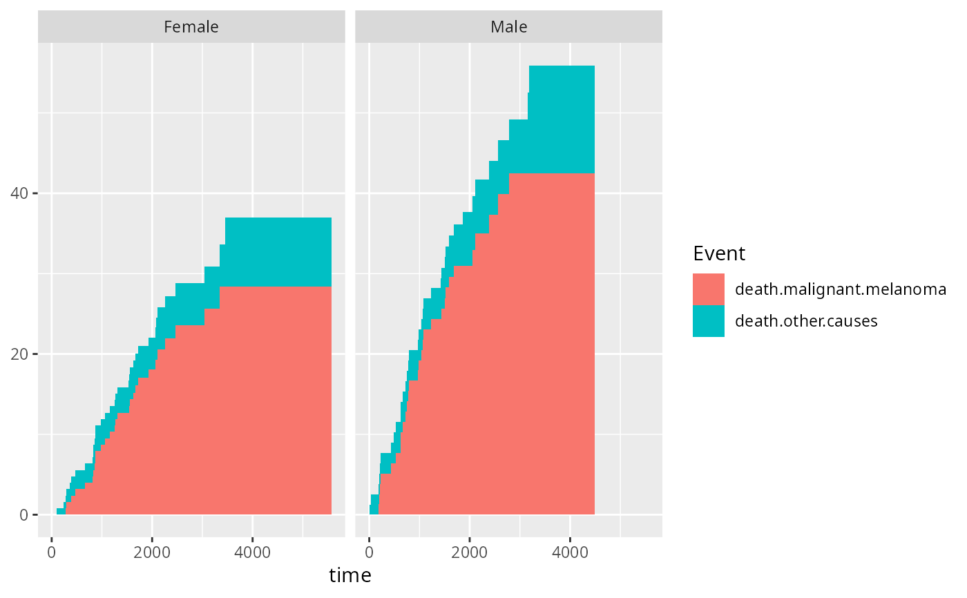
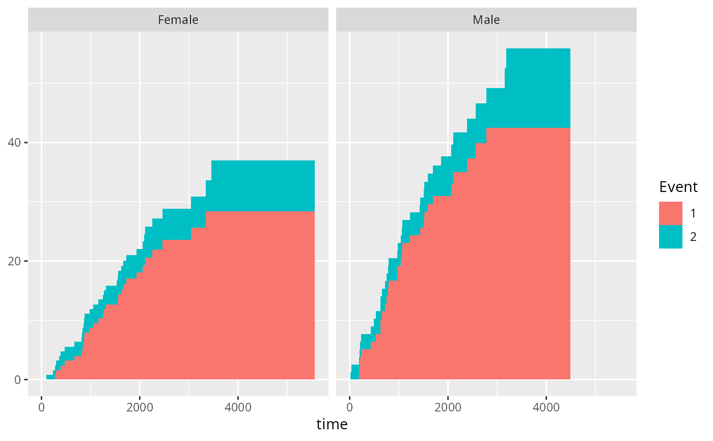
geom_prodlim.RdDraw Kaplan-Meier or Aalen-Johansen curves with optional confidence bands. For competing risks with multiple causes, the default display shows one curve per cause. When `cause = "stacked"`, causes are drawn as stacked filled rectangles instead of step curves with confidence shadows.
Usage
geom_prodlim(
  mapping = NULL,
  data = NULL,
  position = "identity",
  na.rm = FALSE,
  show.legend = NA,
  inherit.aes = TRUE,
  type = "risk",
  cause = NULL,
  conf_int = TRUE,
  conf_int_alpha = 0.2,
  percent = TRUE,
  timeconverter = NULL,
  times = NULL,
  cens.code = "0",
  ...
)
Arguments
- mapping
Set of aesthetic mappings created by [ggplot2::aes()].
- data
Data frame.
- position
Position adjustment.
- na.rm
If `FALSE`, missing values are removed with a warning.
- show.legend
Logical. Should this layer be included in the legends?
- inherit.aes
If `FALSE`, overrides the default aesthetics.
- type
Passed to [prodlim::prodlim()], usually `"risk"` or `"surv"`.
- cause
Cause(s) for competing risks. Can be a vector of causes or the string `"stacked"`.
- conf_int
Logical. Draw confidence intervals.
- conf_int_alpha
Alpha level for confidence shadows.
- percent
Logical. Passed to [prodlim::summary.prodlim()].
- timeconverter
Optional time conversion string.
- times
Optional evaluation times passed to [prodlim::summary.prodlim()].
- cens.code
Censoring code passed to [prodlim::Hist()].
- ...
Further arguments passed to [ggplot2::layer()].
Details
When multiple causes are specified, `fill`/`colour` aesthetics are ignored and replaced by a cause-based mapping so that all causes are shown in a single legend. When `cause = "stacked"`, causes are stacked on top of each other and confidence shadows are not drawn.
Examples
library(riskRegression)
#> riskRegression version 2026.02.13
library(data.table)
library(ggplot2)
#>
#> Attaching package: ‘ggplot2’
#> The following object is masked from ‘package:lava’:
#>
#> vars
data(Melanoma)
# Kaplan-Meier
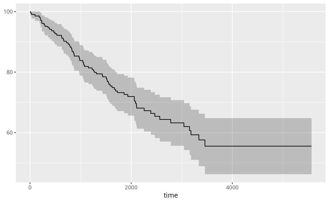
ggplot(data = Melanoma,aes(x = time, event = 1*(status != 0)))+
geom_prodlim(type = "surv")
 # stratified Kaplan-Meier inherited aes
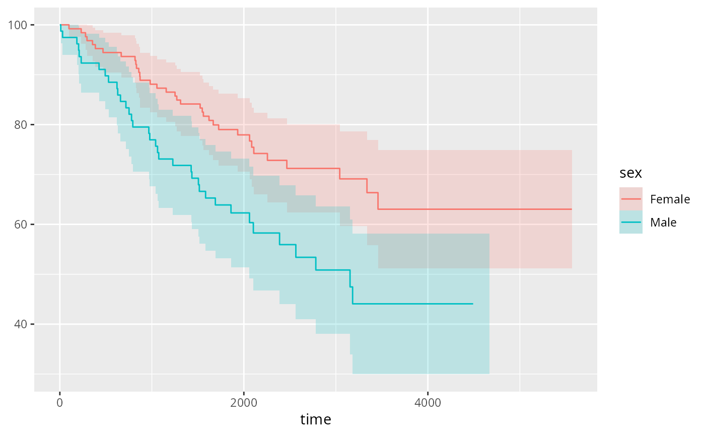
ggplot(data = Melanoma,aes(x = time, event = 1*(status != 0),fill = sex,color = sex))+
geom_prodlim(type = "surv")
# stratified Kaplan-Meier inherited aes
ggplot(data = Melanoma,aes(x = time, event = 1*(status != 0),fill = sex,color = sex))+
geom_prodlim(type = "surv")
 # stratified Kaplan-Meier geom aes
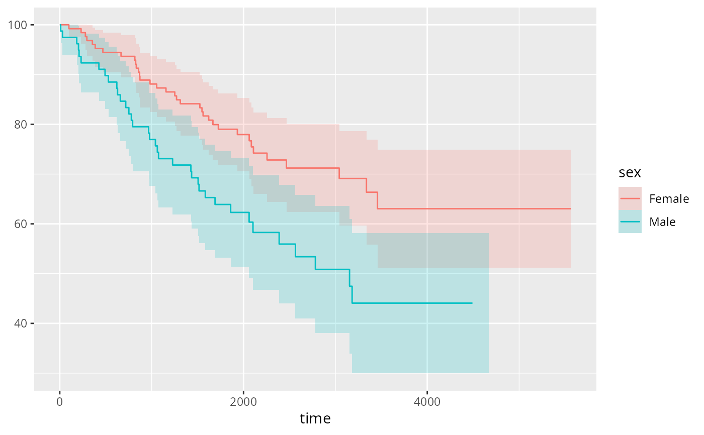
ggplot(data = Melanoma,aes(x = time, event = 1*(status != 0)))+
geom_prodlim(aes(fill = sex,color = sex),type = "surv")
# stratified Kaplan-Meier geom aes
ggplot(data = Melanoma,aes(x = time, event = 1*(status != 0)))+
geom_prodlim(aes(fill = sex,color = sex),type = "surv")
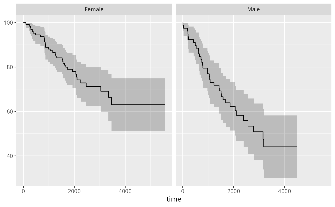
 # facet
ggplot(data = Melanoma,aes(x = time, event = 1*(status != 0)))+
geom_prodlim(type = "surv")+facet_grid(~sex)
# facet
ggplot(data = Melanoma,aes(x = time, event = 1*(status != 0)))+
geom_prodlim(type = "surv")+facet_grid(~sex)
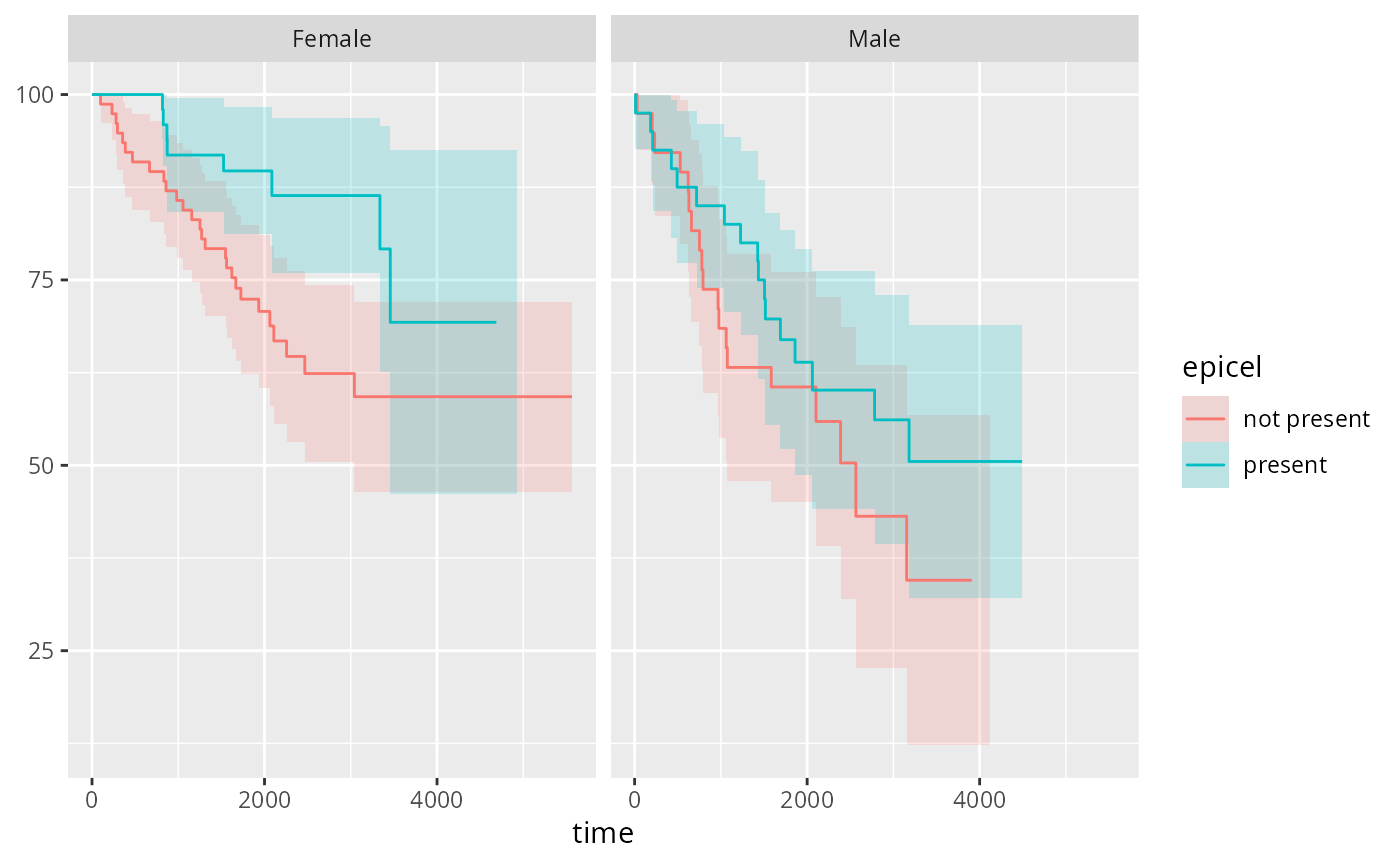
 # stratified and facet
ggplot(data = Melanoma,aes(x = time, event = 1*(status != 0),fill = epicel,color = epicel))+
geom_prodlim(type = "surv")+facet_grid(~sex)
# stratified and facet
ggplot(data = Melanoma,aes(x = time, event = 1*(status != 0),fill = epicel,color = epicel))+
geom_prodlim(type = "surv")+facet_grid(~sex)
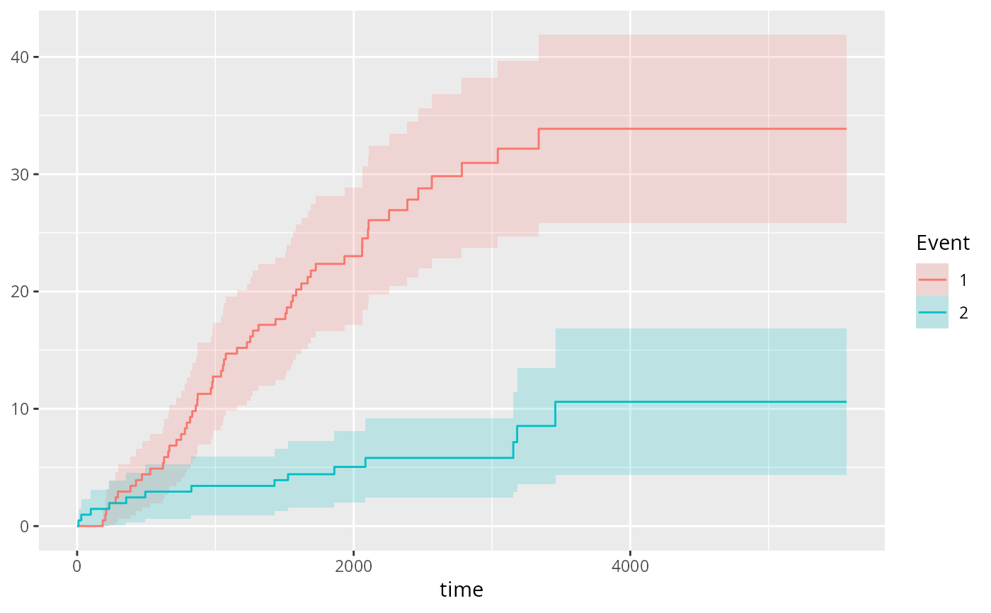
 # Aalen-Johansen
ggplot(data = Melanoma,aes(x = time, event = status))+
geom_prodlim(type = "surv",cause = 1:2)
# Aalen-Johansen
ggplot(data = Melanoma,aes(x = time, event = status))+
geom_prodlim(type = "surv",cause = 1:2)
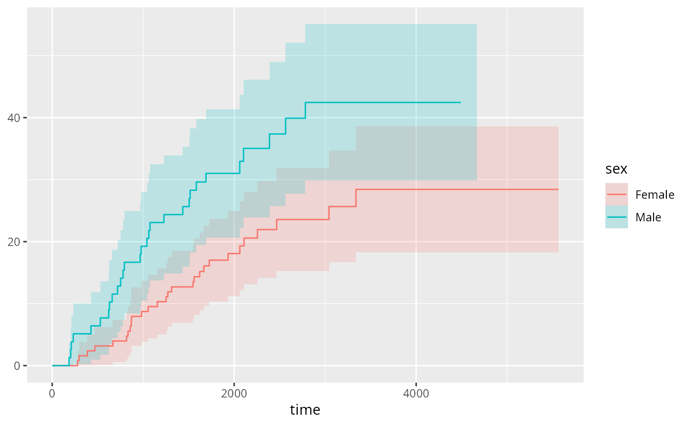
 # stratified Aalen-Johansen inherited aes
ggplot(data = Melanoma,aes(x = time, event = status,fill = sex,color = sex))+
geom_prodlim(type = "surv")
# stratified Aalen-Johansen inherited aes
ggplot(data = Melanoma,aes(x = time, event = status,fill = sex,color = sex))+
geom_prodlim(type = "surv")
 # stratified Aalen-Johansen geom aes
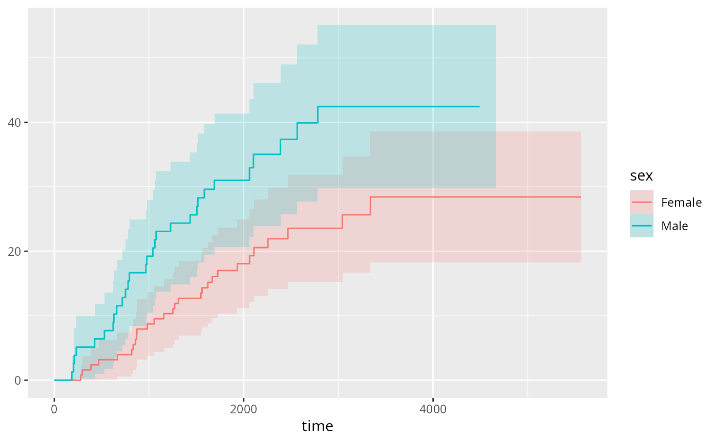
ggplot(data = Melanoma,aes(x = time, event = status))+
geom_prodlim(aes(fill = sex,color = sex),type = "surv")
# stratified Aalen-Johansen geom aes
ggplot(data = Melanoma,aes(x = time, event = status))+
geom_prodlim(aes(fill = sex,color = sex),type = "surv")
 # facet
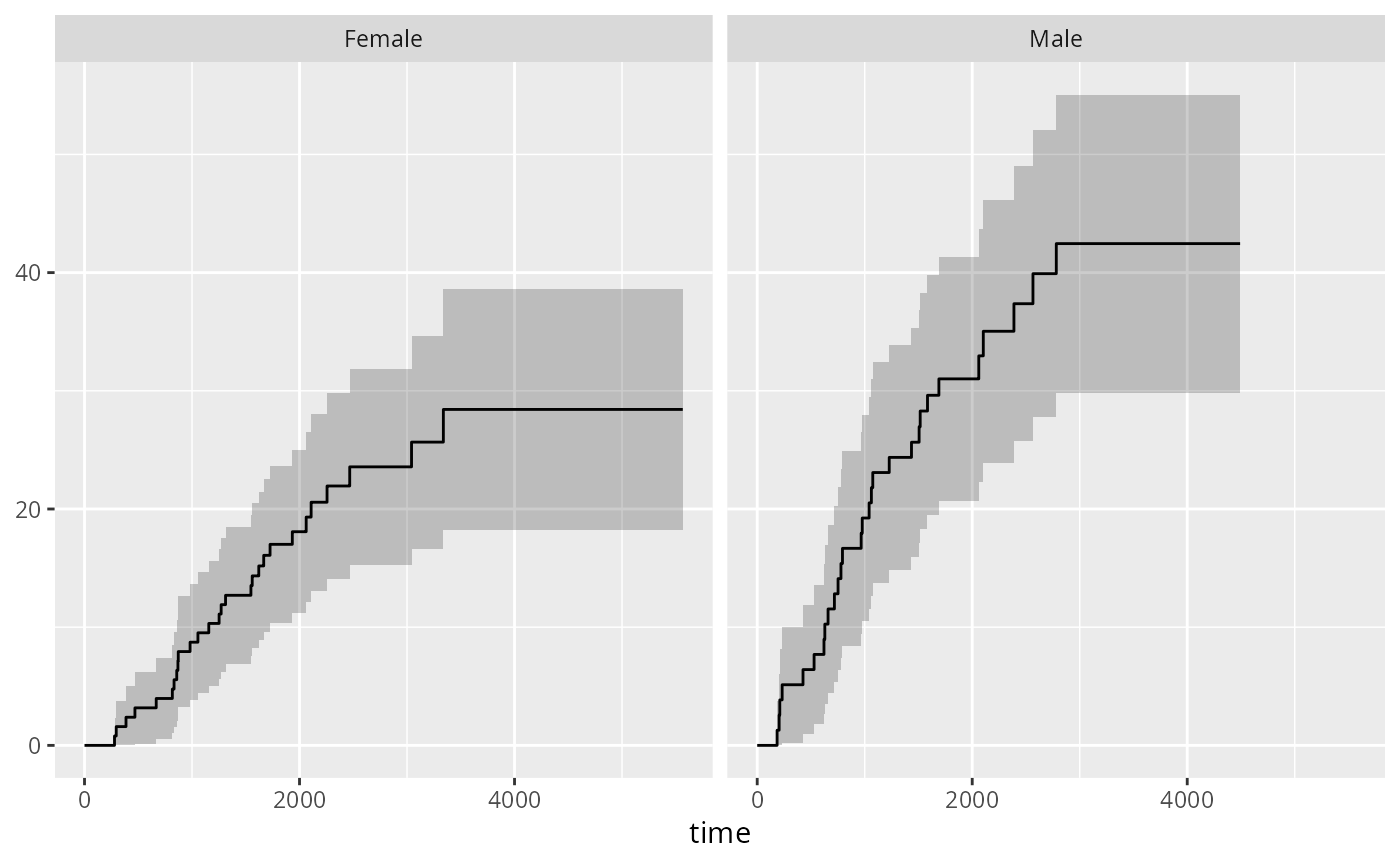
ggplot(data = Melanoma,aes(x = time, event = status))+
geom_prodlim(type = "surv")+facet_grid(~sex)
# facet
ggplot(data = Melanoma,aes(x = time, event = status))+
geom_prodlim(type = "surv")+facet_grid(~sex)
 # stratified and facet
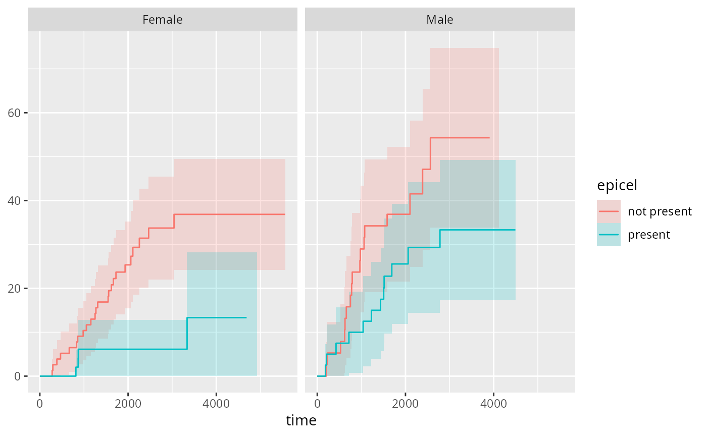
ggplot(data = Melanoma,aes(x = time, event = status,fill = epicel,color = epicel))+
geom_prodlim(type = "surv")+facet_grid(~sex)
# stratified and facet
ggplot(data = Melanoma,aes(x = time, event = status,fill = epicel,color = epicel))+
geom_prodlim(type = "surv")+facet_grid(~sex)
 # stacked
ggplot(data = Melanoma,aes(x = time, event = status))+
geom_prodlim(cause = "stacked")+facet_grid(~sex)
# stacked
ggplot(data = Melanoma,aes(x = time, event = status))+
geom_prodlim(cause = "stacked")+facet_grid(~sex)
 # stacked with cens.code option
ggplot(data = Melanoma,aes(x = time, event = event))+
geom_prodlim(cens.code="censored",cause = "stacked")+facet_grid(~sex)
# stacked with cens.code option
ggplot(data = Melanoma,aes(x = time, event = event))+
geom_prodlim(cens.code="censored",cause = "stacked")+facet_grid(~sex)