Nonparametric estimation in event history analysis. Featuring fast algorithms and user friendly syntax adapted from the survival package. The product limit algorithm is used for right censored data; the self-consistency algorithm for interval censored data.
Usage
prodlim(
  formula,
  data = parent.frame(),
  subset,
  na.action = NULL,
  reverse = FALSE,
  conf.int = 0.95,
  bandwidth = NULL,
  caseweights,
  discrete.level = 3,
  x = TRUE,
  maxiter = 1000,
  grid,
  tol = 7,
  method = c("npmle", "one.step", "impute.midpoint", "impute.right"),
  exact = TRUE,
  type
)
Arguments
- formula
A formula whose left hand side is a
Histobject. In some special cases it can also be aSurvresponse object, see the details section. The right hand side is as usual a linear combination of covariates which may contain at most one continuous factor. Whether or not a covariate is recognized as continuous or discrete depends on its class and on the argumentdiscrete.level. The right hand side may also be used to specify clusters, see the details section.- data
A data.frame in which all the variables of
formulacan be interpreted.- subset
Passed as argument
subsetto functionsubsetwhich applied todatabefore the formula is processed.- na.action
All lines in data with any missing values in the variables of formula are removed.
- reverse
For right censored data, if reverse=TRUE then the censoring distribution is estimated.
- conf.int
The level (between 0 and 1) for two-sided pointwise confidence intervals. Defaults to 0.95. Remark: only plain Wald-type confidence limits are available.
- bandwidth
Smoothing parameter for nearest neighborhoods based on the values of a continuous covariate. See function
neighborhoodfor details.- caseweights
Weights applied to the contribution of each subject to change the number of events and the number at risk. This can be used for bootstrap and survey analysis. Should be a vector of the same length and the same order as
data.- discrete.level
Numeric covariates are treated as factors when their number of unique values exceeds not
discrete.level. Otherwise the product limit method is applied, in overlapping neighborhoods according to the bandwidth.- x
logical value: if
TRUE, the full covariate matrix with is returned in componentmodel.matrix. The reduced matrix contains unique rows of the full covariate matrix and is always returned in componentX.- maxiter
For interval censored data only. Maximal number of iterations to obtain the nonparametric maximum likelihood estimate. Defaults to 1000.
- grid
For interval censored data only. When method=one.step grid for one-step product limit estimate. Defaults to sorted list of unique left and right endpoints of the observed intervals.
- tol
For interval censored data only. Numeric value whose negative exponential is used as convergence criterion for finding the nonparametric maximum likelihood estimate. Defaults to 7 meaning exp(-7).
- method
For interval censored data only. If equal to
"npmle"(the default) use the usual Turnbull algorithm, else the product limit version of the self-consistent estimate.- exact
If TRUE the grid of time points used for estimation includes all the L and R endpoints of the observed intervals.
- type
In two state models either
"surv"for the Kaplan-Meier estimate of the survival function or"risk"for 1-Kaplan-Meier. Default is"surv"whenreverse==FALSEand"risk"whenreverse==TRUE. In competing risks models it has to be"risk"Aalen-Johansen estimate of the cumulative incidence function.
Value
Object of class "prodlim". See print.prodlim, predict.prodlim, predict,
summary.prodlim, plot.prodlim.
Details
The response of formula (ie the left hand side of the `~' operator)
specifies the model.
In two-state models – the classical survival case – the standard
Kaplan-Meier method is applied. For this the response can be specified as a
Surv or as a Hist object. The Hist
function allows you to change the code for censored observations, e.g.
Hist(time,status,cens.code="4").
Besides a slight gain of computing efficiency, there are some extensions that are not included in the current version of the survival package:
(0) The Kaplan-Meier estimator for the censoring times reverse=TRUE
is correctly estimated when there are ties between event and censoring
times.
(1) A conditional version of the kernel smoothed Kaplan-Meier estimator for at most one continuous predictors using nearest neighborhoods (Beran 1981, Stute 1984, Akritas 1994).
(2) For cluster-correlated data the right hand side of formula may
identify a cluster variable. In that case Greenwood's variance
formula is replaced by the formula of Ying and Wei (1994).
(3) Competing risk models can be specified via Hist response
objects in formula.
The Aalen-Johansen estimator is applied for estimating the absolute risk of the competing causes, i.e., the cumulative incidence functions.
Under construction:
(U0) Interval censored event times specified via Hist are used
to find the nonparametric maximum likelihood estimate. Currently this works
only for two-state models and the results should match with those from the
package `Icens'.
(U1) Extensions to more complex multi-states models
(U2) The nonparametric maximum likelihood estimate for interval censored observations of competing risks models.
References
Andersen, Borgan, Gill, Keiding (1993) Springer `Statistical Models Based on Counting Processes'
Akritas (1994) The Annals of Statistics 22, 1299-1327 Nearest neighbor estimation of a bivariate distribution under random censoring.
R Beran (1981) http://anson.ucdavis.edu/~beran/paper.html `Nonparametric regression with randomly censored survival data'
Stute (1984) The Annals of Statistics 12, 917–926 `Asymptotic Normality of Nearest Neighbor Regression Function Estimates'
Ying, Wei (1994) Journal of Multivariate Analysis 50, 17-29 The Kaplan-Meier estimate for dependent failure time observations
Author
Thomas A. Gerds [email protected]
Examples
##---------------------two-state survival model------------
dat <- SimSurv(30)
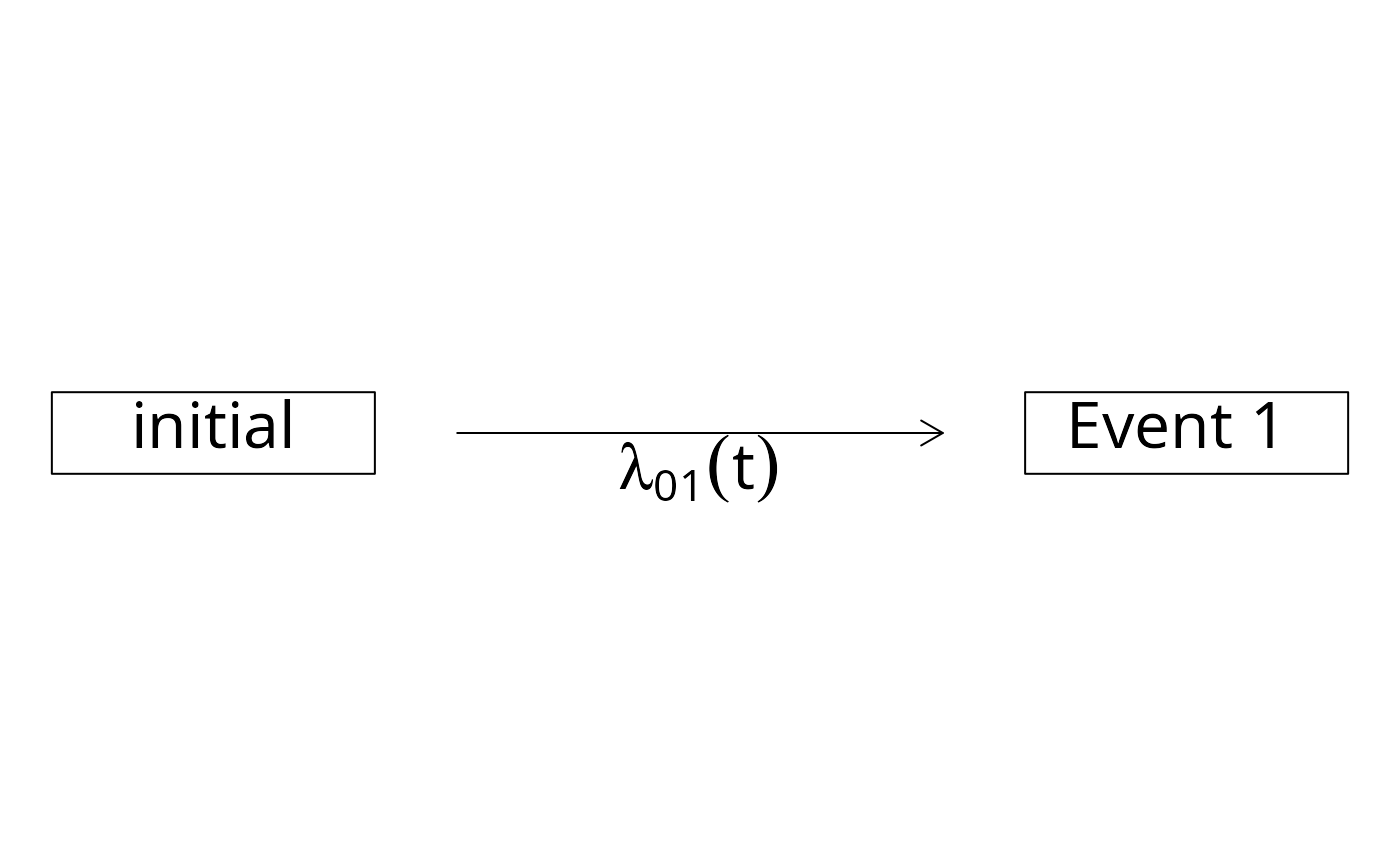
with(dat,plot(Hist(time,status)))
#> Warning: The dimension of the boxes may depend on the current graphical device
#> in the sense that the layout and centering of text may change when you resize the graphical device and call the same plot.
 fit <- prodlim(Hist(time,status)~1,data=dat)
print(fit)
#>
#> Call: prodlim(formula = Hist(time, status) ~ 1, data = dat)
#>
#> Kaplan-Meier estimator for the event time survival function
#>
#> No covariates
#>
#> Right-censored response of a survival model
#>
#> No.Observations: 30
#>
#> Pattern:
#> Freq
#> event 21
#> right.censored 9
plot(fit)
fit <- prodlim(Hist(time,status)~1,data=dat)
print(fit)
#>
#> Call: prodlim(formula = Hist(time, status) ~ 1, data = dat)
#>
#> Kaplan-Meier estimator for the event time survival function
#>
#> No covariates
#>
#> Right-censored response of a survival model
#>
#> No.Observations: 30
#>
#> Pattern:
#> Freq
#> event 21
#> right.censored 9
plot(fit)
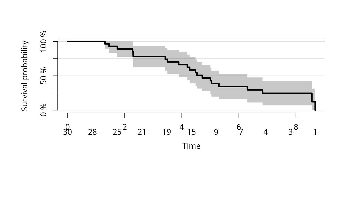 summary(fit)
#> time n.risk n.event n.lost surv se.surv lower upper
#> 1 0.566 30 0 1 1.000 0.0000 1.0000 1.000
#> 2 0.836 29 0 1 1.000 0.0000 1.0000 1.000
#> 3 1.307 28 1 0 0.964 0.0351 0.8955 1.000
#> 4 1.454 27 1 0 0.929 0.0487 0.8332 1.000
#> 5 1.680 26 0 1 0.929 0.0487 0.8332 1.000
#> 6 1.741 25 1 0 0.891 0.0592 0.7754 1.000
#> 7 2.279 24 1 0 0.854 0.0674 0.7222 0.986
#> 8 2.295 23 1 0 0.817 0.0740 0.6721 0.962
#> 9 2.298 22 1 0 0.780 0.0794 0.6243 0.936
#> 10 3.217 21 0 1 0.780 0.0794 0.6243 0.936
#> 11 3.422 20 1 0 0.741 0.0845 0.5754 0.907
#> 12 3.496 19 1 0 0.702 0.0886 0.5284 0.876
#> 13 3.894 18 1 0 0.663 0.0918 0.4830 0.843
#> 14 4.196 17 1 0 0.624 0.0944 0.4391 0.809
#> 15 4.276 16 1 0 0.585 0.0962 0.3965 0.774
#> 16 4.482 15 1 0 0.546 0.0974 0.3552 0.737
#> 17 4.532 14 1 0 0.507 0.0979 0.3151 0.699
#> 18 4.718 13 1 0 0.468 0.0978 0.2763 0.660
#> 19 5.004 12 1 0 0.429 0.0971 0.2386 0.619
#> 20 5.007 11 0 1 0.429 0.0971 0.2386 0.619
#> 21 5.039 10 1 0 0.386 0.0964 0.1971 0.575
#> 22 5.302 9 1 0 0.343 0.0948 0.1574 0.529
#> 23 5.936 8 0 1 0.343 0.0948 0.1574 0.529
#> 24 6.299 7 1 0 0.294 0.0931 0.1118 0.477
#> 25 6.831 6 1 0 0.245 0.0895 0.0696 0.421
#> 26 6.852 5 0 1 0.245 0.0895 0.0696 0.421
#> 27 7.590 4 0 1 0.245 0.0895 0.0696 0.421
#> 28 8.529 3 0 1 0.245 0.0895 0.0696 0.421
#> 29 8.560 2 1 0 0.123 0.0976 0.0000 0.314
#> 30 8.677 1 1 0 0.000 NaN 0.0000 0.000
quantile(fit)
#> Quantiles of the event time distribution based on the Kaplan-Meier method.
#>
#> Table of quantiles and corresponding confidence limits:
#> q quantile lower upper
#> <num> <num> <num> <num>
#> 1: 0.00 NA NA NA
#> 2: 0.25 6.8 5.0 NA
#> 3: 0.50 4.7 3.9 6.3
#> 4: 0.75 3.4 2.3 4.5
#> 5: 1.00 1.3 1.3 2.3
#>
#>
#> Median with interquartile range (IQR):
#> Median (IQR)
#> <char>
#> 1: 4.72 (3.42;6.83)
## Subset
fit1a <- prodlim(Hist(time,status)~1,data=dat,subset=dat$X1==1)
fit1b <- prodlim(Hist(time,status)~1,data=dat,subset=dat$X1==1 & dat$X2>0)
## --------------------clustered data---------------------
library(survival)
cdat <- cbind(SimSurv(30),patnr=sample(1:5,size=30,replace=TRUE))
fit <- prodlim(Hist(time,status)~cluster(patnr),data=cdat)
print(fit)
#>
#> Call: prodlim(formula = Hist(time, status) ~ cluster(patnr), data = cdat)
#>
#> Kaplan-Meier estimator for the event time survival function
#>
#>
#> Cluster-correlated data:
#>
#> cluster variable: patnr
#> No covariates
#>
#> Right-censored response of a survival model
#>
#> No.Observations: 30
#>
#> Pattern:
#> Freq
#> event 11
#> right.censored 19
plot(fit)
summary(fit)
#> time n.risk n.event n.lost surv se.surv lower upper
#> 1 0.566 30 0 1 1.000 0.0000 1.0000 1.000
#> 2 0.836 29 0 1 1.000 0.0000 1.0000 1.000
#> 3 1.307 28 1 0 0.964 0.0351 0.8955 1.000
#> 4 1.454 27 1 0 0.929 0.0487 0.8332 1.000
#> 5 1.680 26 0 1 0.929 0.0487 0.8332 1.000
#> 6 1.741 25 1 0 0.891 0.0592 0.7754 1.000
#> 7 2.279 24 1 0 0.854 0.0674 0.7222 0.986
#> 8 2.295 23 1 0 0.817 0.0740 0.6721 0.962
#> 9 2.298 22 1 0 0.780 0.0794 0.6243 0.936
#> 10 3.217 21 0 1 0.780 0.0794 0.6243 0.936
#> 11 3.422 20 1 0 0.741 0.0845 0.5754 0.907
#> 12 3.496 19 1 0 0.702 0.0886 0.5284 0.876
#> 13 3.894 18 1 0 0.663 0.0918 0.4830 0.843
#> 14 4.196 17 1 0 0.624 0.0944 0.4391 0.809
#> 15 4.276 16 1 0 0.585 0.0962 0.3965 0.774
#> 16 4.482 15 1 0 0.546 0.0974 0.3552 0.737
#> 17 4.532 14 1 0 0.507 0.0979 0.3151 0.699
#> 18 4.718 13 1 0 0.468 0.0978 0.2763 0.660
#> 19 5.004 12 1 0 0.429 0.0971 0.2386 0.619
#> 20 5.007 11 0 1 0.429 0.0971 0.2386 0.619
#> 21 5.039 10 1 0 0.386 0.0964 0.1971 0.575
#> 22 5.302 9 1 0 0.343 0.0948 0.1574 0.529
#> 23 5.936 8 0 1 0.343 0.0948 0.1574 0.529
#> 24 6.299 7 1 0 0.294 0.0931 0.1118 0.477
#> 25 6.831 6 1 0 0.245 0.0895 0.0696 0.421
#> 26 6.852 5 0 1 0.245 0.0895 0.0696 0.421
#> 27 7.590 4 0 1 0.245 0.0895 0.0696 0.421
#> 28 8.529 3 0 1 0.245 0.0895 0.0696 0.421
#> 29 8.560 2 1 0 0.123 0.0976 0.0000 0.314
#> 30 8.677 1 1 0 0.000 NaN 0.0000 0.000
quantile(fit)
#> Quantiles of the event time distribution based on the Kaplan-Meier method.
#>
#> Table of quantiles and corresponding confidence limits:
#> q quantile lower upper
#> <num> <num> <num> <num>
#> 1: 0.00 NA NA NA
#> 2: 0.25 6.8 5.0 NA
#> 3: 0.50 4.7 3.9 6.3
#> 4: 0.75 3.4 2.3 4.5
#> 5: 1.00 1.3 1.3 2.3
#>
#>
#> Median with interquartile range (IQR):
#> Median (IQR)
#> <char>
#> 1: 4.72 (3.42;6.83)
## Subset
fit1a <- prodlim(Hist(time,status)~1,data=dat,subset=dat$X1==1)
fit1b <- prodlim(Hist(time,status)~1,data=dat,subset=dat$X1==1 & dat$X2>0)
## --------------------clustered data---------------------
library(survival)
cdat <- cbind(SimSurv(30),patnr=sample(1:5,size=30,replace=TRUE))
fit <- prodlim(Hist(time,status)~cluster(patnr),data=cdat)
print(fit)
#>
#> Call: prodlim(formula = Hist(time, status) ~ cluster(patnr), data = cdat)
#>
#> Kaplan-Meier estimator for the event time survival function
#>
#>
#> Cluster-correlated data:
#>
#> cluster variable: patnr
#> No covariates
#>
#> Right-censored response of a survival model
#>
#> No.Observations: 30
#>
#> Pattern:
#> Freq
#> event 11
#> right.censored 19
plot(fit)
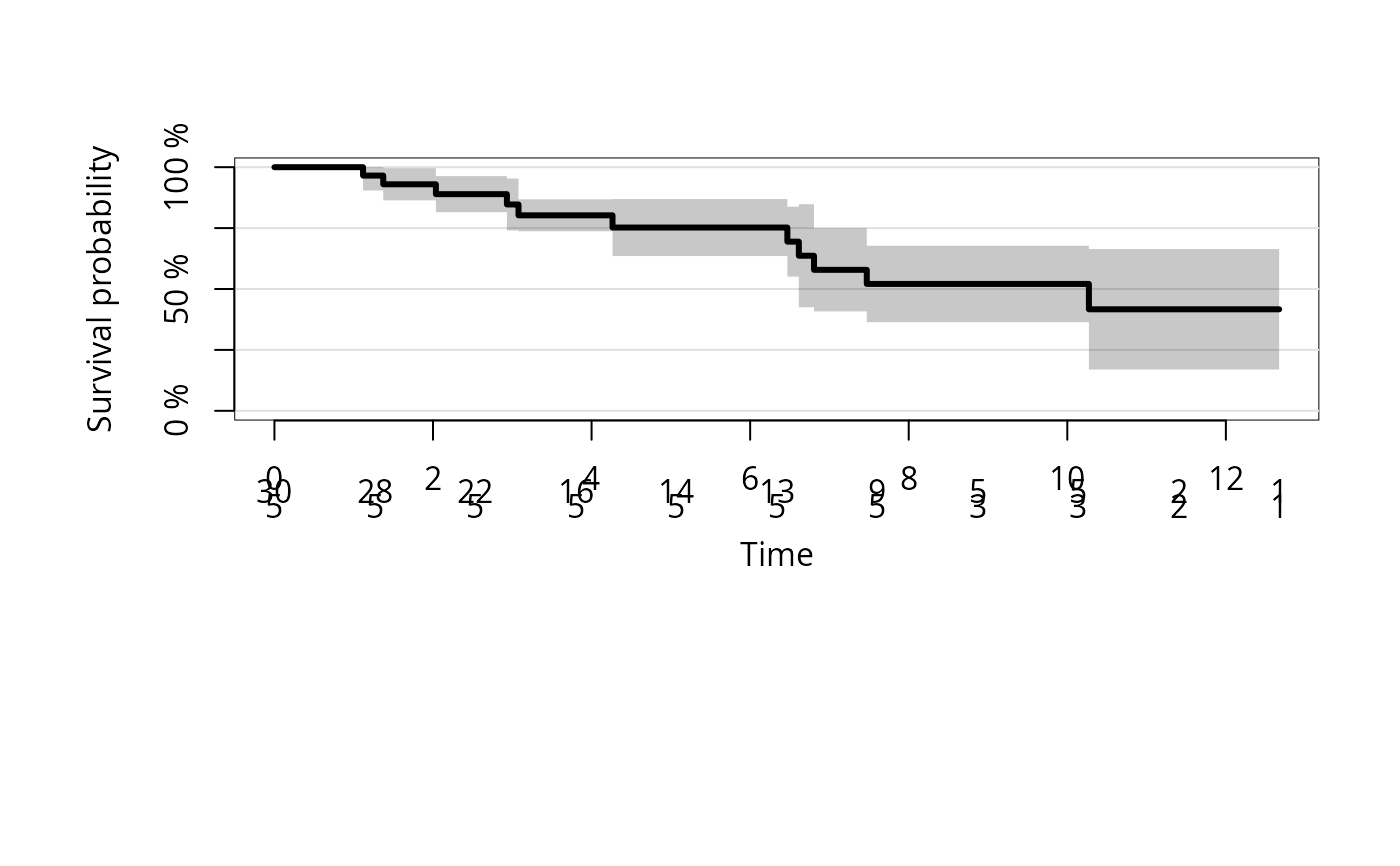 summary(fit)
#> time n.risk n.event n.lost patnr.n.risk patnr.n.event patnr.n.lost surv
#> 1 0.95 30 0 1 5 0 0 1.000
#> 2 1.12 29 1 0 5 1 0 0.966
#> 3 1.32 28 0 1 5 0 0 0.966
#> 4 1.37 27 1 0 5 1 0 0.930
#> 5 1.57 26 0 1 5 0 0 0.930
#> 6 1.72 25 0 1 5 0 0 0.930
#> 7 1.74 24 0 1 5 0 0 0.930
#> 8 2.04 23 1 0 5 1 0 0.889
#> 9 2.92 22 0 1 5 0 0 0.889
#> 10 2.93 21 1 0 5 1 0 0.847
#> 11 3.06 20 0 1 5 0 0 0.847
#> 12 3.08 19 1 0 5 1 0 0.802
#> 13 3.37 18 0 1 5 0 0 0.802
#> 14 3.63 17 0 1 5 0 0 0.802
#> 15 4.26 16 1 0 5 1 0 0.752
#> 16 4.42 15 0 1 5 0 0 0.752
#> 17 6.03 14 0 1 5 0 0 0.752
#> 18 6.47 13 1 0 5 1 0 0.694
#> 19 6.61 12 1 0 5 1 0 0.637
#> 20 6.81 11 1 0 5 1 0 0.579
#> 21 7.47 10 1 0 5 1 0 0.521
#> 22 8.02 9 0 1 5 0 1 0.521
#> 23 8.23 8 0 1 4 0 0 0.521
#> 24 8.63 7 0 1 4 0 1 0.521
#> 25 8.86 6 0 1 3 0 0 0.521
#> 26 10.27 5 1 0 3 1 0 0.417
#> 27 10.95 4 0 1 2 0 0 0.417
#> 28 11.31 3 0 1 2 0 0 0.417
#> 29 11.46 2 0 1 2 0 1 0.417
#> 30 12.67 1 0 1 1 0 0 0.417
#> se.surv lower upper
#> 1 0.0000 1.000 1.000
#> 2 0.0312 0.904 1.000
#> 3 0.0312 0.904 1.000
#> 4 0.0337 0.864 0.996
#> 5 0.0337 0.864 0.996
#> 6 0.0337 0.864 0.996
#> 7 0.0337 0.864 0.996
#> 8 0.0378 0.815 0.963
#> 9 0.0378 0.815 0.963
#> 10 0.0544 0.740 0.954
#> 11 0.0544 0.740 0.954
#> 12 0.0334 0.737 0.868
#> 13 0.0334 0.737 0.868
#> 14 0.0334 0.737 0.868
#> 15 0.0597 0.635 0.869
#> 16 0.0597 0.635 0.869
#> 17 0.0597 0.635 0.869
#> 18 0.0732 0.551 0.838
#> 19 0.1079 0.425 0.848
#> 20 0.0870 0.408 0.749
#> 21 0.0800 0.364 0.678
#> 22 0.0800 0.364 0.678
#> 23 0.0800 0.364 0.678
#> 24 0.0800 0.364 0.678
#> 25 0.0800 0.364 0.678
#> 26 0.1261 0.169 0.664
#> 27 0.1261 0.169 0.664
#> 28 0.1261 0.169 0.664
#> 29 0.1261 0.169 0.664
#> 30 0.1261 0.169 0.664
##-----------compare Kaplan-Meier to survival package---------
dat <- SimSurv(30)
pfit <- prodlim(Surv(time,status)~1,data=dat)
pfit <- prodlim(Hist(time,status)~1,data=dat) ## same thing
sfit <- survfit(Surv(time,status)~1,data=dat,conf.type="plain")
## same result for the survival distribution function
all(round(pfit$surv,12)==round(sfit$surv,12))
#> [1] TRUE
summary(pfit,digits=3)
#> time n.risk n.event n.lost surv se.surv lower upper
#> 1 0.321 30 0 1 1.000 0.0000 1.000 1.000
#> 2 0.707 29 0 1 1.000 0.0000 1.000 1.000
#> 3 1.118 28 0 1 1.000 0.0000 1.000 1.000
#> 4 1.479 27 0 1 1.000 0.0000 1.000 1.000
#> 5 1.907 26 0 1 1.000 0.0000 1.000 1.000
#> 6 2.180 25 1 0 0.960 0.0392 0.883 1.000
#> 7 2.275 24 1 0 0.920 0.0543 0.814 1.000
#> 8 2.602 23 1 0 0.880 0.0650 0.753 1.000
#> 9 2.723 22 1 0 0.840 0.0733 0.696 0.984
#> 10 4.320 21 0 1 0.840 0.0733 0.696 0.984
#> 11 4.719 20 1 0 0.798 0.0808 0.640 0.956
#> 12 4.736 19 1 0 0.756 0.0868 0.586 0.926
#> 13 4.979 18 1 0 0.714 0.0916 0.535 0.893
#> 14 5.841 17 1 0 0.672 0.0953 0.485 0.859
#> 15 6.038 16 1 0 0.630 0.0982 0.438 0.822
#> 16 6.153 15 1 0 0.588 0.1002 0.392 0.784
#> 17 6.281 14 0 1 0.588 0.1002 0.392 0.784
#> 18 6.298 13 1 0 0.543 0.1022 0.342 0.743
#> 19 6.317 12 1 0 0.498 0.1032 0.295 0.700
#> 20 6.493 11 0 1 0.498 0.1032 0.295 0.700
#> 21 6.534 10 0 1 0.498 0.1032 0.295 0.700
#> 22 7.065 9 1 0 0.442 0.1055 0.235 0.649
#> 23 8.066 8 1 0 0.387 0.1058 0.180 0.594
#> 24 8.385 7 0 1 0.387 0.1058 0.180 0.594
#> 25 9.337 6 0 1 0.387 0.1058 0.180 0.594
#> 26 9.535 5 0 1 0.387 0.1058 0.180 0.594
#> 27 10.292 4 0 1 0.387 0.1058 0.180 0.594
#> 28 11.982 3 0 1 0.387 0.1058 0.180 0.594
#> 29 14.529 2 1 0 0.193 0.1467 0.000 0.481
#> 30 14.678 1 0 1 0.193 0.1467 0.000 0.481
summary(sfit,times=quantile(unique(dat$time)))
#> Call: survfit(formula = Surv(time, status) ~ 1, data = dat, conf.type = "plain")
#>
#> time n.risk n.event survival std.err lower 95% CI upper 95% CI
#> 0.321 30 0 1.000 0.0000 1.000 1.000
#> 2.632 22 3 0.880 0.0650 0.753 1.000
#> 6.096 15 6 0.630 0.0982 0.438 0.822
#> 7.816 8 4 0.442 0.1055 0.235 0.649
#> 14.678 1 2 0.193 0.1467 0.000 0.481
##-----------estimating the censoring survival function----------------
rdat <- data.frame(time=c(1,2,3,3,3,4,5,5,6,7),status=c(1,0,0,1,0,1,0,1,1,0))
rpfit <- prodlim(Hist(time,status)~1,data=rdat,reverse=TRUE)
rsfit <- survfit(Surv(time,1-status)~1,data=rdat,conf.type="plain")
## When there are ties between times at which events are observed
## times at which subjects are right censored, then the convention
## is that events come first. This is not obeyed by the above call to survfit,
## and hence only prodlim delivers the correct reverse Kaplan-Meier:
cbind("Wrong:"=rsfit$surv,"Correct:"=rpfit$surv)
#> Wrong: Correct:
#> [1,] 1.0000000 1.0000000
#> [2,] 0.8888889 0.8888889
#> [3,] 0.6666667 0.6349206
#> [4,] 0.6666667 0.6349206
#> [5,] 0.5000000 0.4232804
#> [6,] 0.5000000 0.4232804
#> [7,] 0.0000000 0.0000000
##---------------- quantiles of the potential followup time-----
G=prodlim(Hist(time,status)~X1,data=dat,reverse=TRUE)
quantile(G)
#> Quantiles of the potential follow up time distribution based on the Kaplan-Meier method
#> applied to the censored times reversing the roles of event status and censored.
#>
#> Table of quantiles and corresponding confidence limits:
#> X1 q quantile lower upper
#> <num> <num> <num> <num> <num>
#> 1: 0 0.00 NA NA NA
#> 2: 0 0.25 NA 11.98 NA
#> 3: 0 0.50 11.98 6.49 NA
#> 4: 0 0.75 6.49 1.12 12.0
#> 5: 0 1.00 0.71 0.71 6.5
#> 6: 1 0.00 NA NA NA
#> 7: 1 0.25 9.53 8.39 NA
#> 8: 1 0.50 9.34 4.32 9.5
#> 9: 1 0.75 4.32 1.48 9.3
#> 10: 1 1.00 0.32 0.32 1.9
#>
#>
#> Median with interquartile range (IQR):
#> X1 Median (IQR)
#> <num> <char>
#> 1: 0 11.98 (6.49;NA)
#> 2: 1 9.34 (4.32;9.53)
##-------------------stratified Kaplan-Meier---------------------
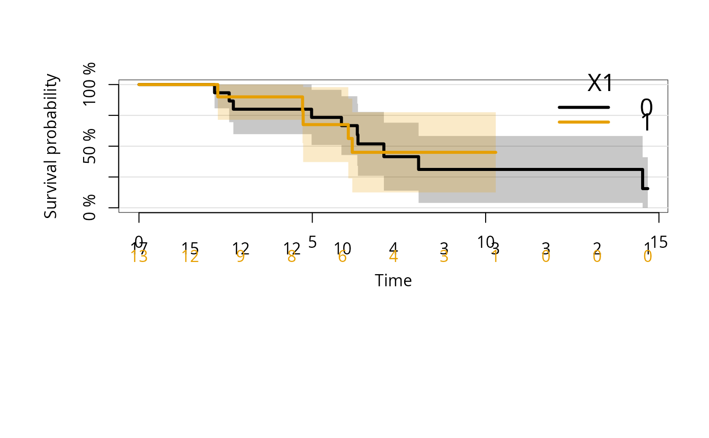
stratfit <- prodlim(Surv(time,status)~X1,data=dat)
summary(stratfit)
#> X1 time n.risk n.event n.lost surv se.surv lower upper
#> 1 0 0.321 17 0 0 1.000 0.0000 1.0000 1.000
#> 2 0 0.707 17 0 1 1.000 0.0000 1.0000 1.000
#> 3 0 1.118 16 0 1 1.000 0.0000 1.0000 1.000
#> 4 0 1.479 15 0 0 1.000 0.0000 1.0000 1.000
#> 5 0 1.907 15 0 0 1.000 0.0000 1.0000 1.000
#> 6 0 2.180 15 1 0 0.933 0.0644 0.8071 1.000
#> 7 0 2.275 14 0 0 0.933 0.0644 0.8071 1.000
#> 8 0 2.602 14 1 0 0.867 0.0878 0.6946 1.000
#> 9 0 2.723 13 1 0 0.800 0.1033 0.5976 1.000
#> 10 0 4.320 12 0 0 0.800 0.1033 0.5976 1.000
#> 11 0 4.719 12 0 0 0.800 0.1033 0.5976 1.000
#> 12 0 4.736 12 0 0 0.800 0.1033 0.5976 1.000
#> 13 0 4.979 12 1 0 0.733 0.1142 0.5095 0.957
#> 14 0 5.841 11 1 0 0.667 0.1217 0.4281 0.905
#> 15 0 6.038 10 0 0 0.667 0.1217 0.4281 0.905
#> 16 0 6.153 10 0 0 0.667 0.1217 0.4281 0.905
#> 17 0 6.281 10 0 1 0.667 0.1217 0.4281 0.905
#> 18 0 6.298 9 1 0 0.593 0.1288 0.3402 0.845
#> 19 0 6.317 8 1 0 0.519 0.1323 0.2593 0.778
#> 20 0 6.493 7 0 1 0.519 0.1323 0.2593 0.778
#> 21 0 6.534 6 0 1 0.519 0.1323 0.2593 0.778
#> 22 0 7.065 5 1 0 0.415 0.1407 0.1390 0.691
#> 23 0 8.066 4 1 0 0.311 0.1386 0.0395 0.583
#> 24 0 8.385 3 0 0 0.311 0.1386 0.0395 0.583
#> 25 0 9.337 3 0 0 0.311 0.1386 0.0395 0.583
#> 26 0 9.535 3 0 0 0.311 0.1386 0.0395 0.583
#> 27 0 10.292 3 0 0 0.311 0.1386 0.0395 0.583
#> 28 0 11.982 3 0 1 0.311 0.1386 0.0395 0.583
#> 29 0 14.529 2 1 0 0.156 0.1300 0.0000 0.410
#> 30 0 14.678 1 0 1 0.156 0.1300 0.0000 0.410
#> 31 1 0.321 13 0 1 1.000 0.0000 1.0000 1.000
#> 32 1 0.707 12 0 0 1.000 0.0000 1.0000 1.000
#> 33 1 1.118 12 0 0 1.000 0.0000 1.0000 1.000
#> 34 1 1.479 12 0 1 1.000 0.0000 1.0000 1.000
#> 35 1 1.907 11 0 1 1.000 0.0000 1.0000 1.000
#> 36 1 2.180 10 0 0 1.000 0.0000 1.0000 1.000
#> 37 1 2.275 10 1 0 0.900 0.0949 0.7141 1.000
#> 38 1 2.602 9 0 0 0.900 0.0949 0.7141 1.000
#> 39 1 2.723 9 0 0 0.900 0.0949 0.7141 1.000
#> 40 1 4.320 9 0 1 0.900 0.0949 0.7141 1.000
#> 41 1 4.719 8 1 0 0.787 0.1340 0.5248 1.000
#> 42 1 4.736 7 1 0 0.675 0.1551 0.3711 0.979
#> 43 1 4.979 6 0 0 0.675 0.1551 0.3711 0.979
#> 44 1 5.841 6 0 0 0.675 0.1551 0.3711 0.979
#> 45 1 6.038 6 1 0 0.562 0.1651 0.2390 0.886
#> 46 1 6.153 5 1 0 0.450 0.1660 0.1246 0.775
#> 47 1 6.281 4 0 0 0.450 0.1660 0.1246 0.775
#> 48 1 6.298 4 0 0 0.450 0.1660 0.1246 0.775
#> 49 1 6.317 4 0 0 0.450 0.1660 0.1246 0.775
#> 50 1 6.493 4 0 0 0.450 0.1660 0.1246 0.775
#> 51 1 6.534 4 0 0 0.450 0.1660 0.1246 0.775
#> 52 1 7.065 4 0 0 0.450 0.1660 0.1246 0.775
#> 53 1 8.066 4 0 0 0.450 0.1660 0.1246 0.775
#> 54 1 8.385 4 0 1 0.450 0.1660 0.1246 0.775
#> 55 1 9.337 3 0 1 0.450 0.1660 0.1246 0.775
#> 56 1 9.535 2 0 1 0.450 0.1660 0.1246 0.775
#> 57 1 10.292 1 0 1 0.450 0.1660 0.1246 0.775
#> 58 1 11.982 0 0 0 NA NA NA NA
#> 59 1 14.529 0 0 0 NA NA NA NA
#> 60 1 14.678 0 0 0 NA NA NA NA
summary(stratfit,intervals=TRUE)
#> X1 time0 time1 n.risk n.event n.lost surv se.surv lower upper
#> 1 0 0.00 0.321 17 0 0 1.000 0.0000 1.0000 1.000
#> 2 0 0.32 0.707 17 0 0 1.000 0.0000 1.0000 1.000
#> 3 0 0.71 1.118 17 0 1 1.000 0.0000 1.0000 1.000
#> 4 0 1.12 1.479 16 0 1 1.000 0.0000 1.0000 1.000
#> 5 0 1.48 1.907 15 0 0 1.000 0.0000 1.0000 1.000
#> 6 0 1.91 2.180 15 0 0 0.933 0.0644 0.8071 1.000
#> 7 0 2.18 2.275 15 1 0 0.933 0.0644 0.8071 1.000
#> 8 0 2.27 2.602 14 0 0 0.867 0.0878 0.6946 1.000
#> 9 0 2.60 2.723 14 1 0 0.800 0.1033 0.5976 1.000
#> 10 0 2.72 4.320 13 1 0 0.800 0.1033 0.5976 1.000
#> 11 0 4.32 4.719 12 0 0 0.800 0.1033 0.5976 1.000
#> 12 0 4.72 4.736 12 0 0 0.800 0.1033 0.5976 1.000
#> 13 0 4.74 4.979 12 0 0 0.733 0.1142 0.5095 0.957
#> 14 0 4.98 5.841 12 1 0 0.667 0.1217 0.4281 0.905
#> 15 0 5.84 6.038 11 1 0 0.667 0.1217 0.4281 0.905
#> 16 0 6.04 6.153 10 0 0 0.667 0.1217 0.4281 0.905
#> 17 0 6.15 6.281 10 0 0 0.667 0.1217 0.4281 0.905
#> 18 0 6.28 6.298 10 0 1 0.593 0.1288 0.3402 0.845
#> 19 0 6.30 6.317 9 1 0 0.519 0.1323 0.2593 0.778
#> 20 0 6.32 6.493 8 1 0 0.519 0.1323 0.2593 0.778
#> 21 0 6.49 6.534 7 0 1 0.519 0.1323 0.2593 0.778
#> 22 0 6.53 7.065 6 0 1 0.415 0.1407 0.1390 0.691
#> 23 0 7.06 8.066 5 1 0 0.311 0.1386 0.0395 0.583
#> 24 0 8.07 8.385 4 1 0 0.311 0.1386 0.0395 0.583
#> 25 0 8.39 9.337 3 0 0 0.311 0.1386 0.0395 0.583
#> 26 0 9.34 9.535 3 0 0 0.311 0.1386 0.0395 0.583
#> 27 0 9.53 10.292 3 0 0 0.311 0.1386 0.0395 0.583
#> 28 0 10.29 11.982 3 0 0 0.311 0.1386 0.0395 0.583
#> 29 0 11.98 14.529 3 0 1 0.156 0.1300 0.0000 0.410
#> 30 0 14.53 14.678 2 1 0 0.156 0.1300 0.0000 0.410
#> 31 1 0.00 0.321 13 0 0 1.000 0.0000 1.0000 1.000
#> 32 1 0.32 0.707 13 0 1 1.000 0.0000 1.0000 1.000
#> 33 1 0.71 1.118 12 0 0 1.000 0.0000 1.0000 1.000
#> 34 1 1.12 1.479 12 0 0 1.000 0.0000 1.0000 1.000
#> 35 1 1.48 1.907 12 0 1 1.000 0.0000 1.0000 1.000
#> 36 1 1.91 2.180 11 0 1 1.000 0.0000 1.0000 1.000
#> 37 1 2.18 2.275 10 0 0 0.900 0.0949 0.7141 1.000
#> 38 1 2.27 2.602 10 1 0 0.900 0.0949 0.7141 1.000
#> 39 1 2.60 2.723 9 0 0 0.900 0.0949 0.7141 1.000
#> 40 1 2.72 4.320 9 0 0 0.900 0.0949 0.7141 1.000
#> 41 1 4.32 4.719 9 0 1 0.787 0.1340 0.5248 1.000
#> 42 1 4.72 4.736 8 1 0 0.675 0.1551 0.3711 0.979
#> 43 1 4.74 4.979 7 1 0 0.675 0.1551 0.3711 0.979
#> 44 1 4.98 5.841 6 0 0 0.675 0.1551 0.3711 0.979
#> 45 1 5.84 6.038 6 0 0 0.562 0.1651 0.2390 0.886
#> 46 1 6.04 6.153 6 1 0 0.450 0.1660 0.1246 0.775
#> 47 1 6.15 6.281 5 1 0 0.450 0.1660 0.1246 0.775
#> 48 1 6.28 6.298 4 0 0 0.450 0.1660 0.1246 0.775
#> 49 1 6.30 6.317 4 0 0 0.450 0.1660 0.1246 0.775
#> 50 1 6.32 6.493 4 0 0 0.450 0.1660 0.1246 0.775
#> 51 1 6.49 6.534 4 0 0 0.450 0.1660 0.1246 0.775
#> 52 1 6.53 7.065 4 0 0 0.450 0.1660 0.1246 0.775
#> 53 1 7.06 8.066 4 0 0 0.450 0.1660 0.1246 0.775
#> 54 1 8.07 8.385 4 0 0 0.450 0.1660 0.1246 0.775
#> 55 1 8.39 9.337 4 0 1 0.450 0.1660 0.1246 0.775
#> 56 1 9.34 9.535 3 0 1 0.450 0.1660 0.1246 0.775
#> 57 1 9.53 10.292 2 0 1 0.450 0.1660 0.1246 0.775
#> 58 1 10.29 11.982 1 0 1 NA NA NA NA
#> 59 1 11.98 14.529 0 0 0 NA NA NA NA
#> 60 1 14.53 14.678 0 0 0 NA NA NA NA
plot(stratfit)
summary(fit)
#> time n.risk n.event n.lost patnr.n.risk patnr.n.event patnr.n.lost surv
#> 1 0.95 30 0 1 5 0 0 1.000
#> 2 1.12 29 1 0 5 1 0 0.966
#> 3 1.32 28 0 1 5 0 0 0.966
#> 4 1.37 27 1 0 5 1 0 0.930
#> 5 1.57 26 0 1 5 0 0 0.930
#> 6 1.72 25 0 1 5 0 0 0.930
#> 7 1.74 24 0 1 5 0 0 0.930
#> 8 2.04 23 1 0 5 1 0 0.889
#> 9 2.92 22 0 1 5 0 0 0.889
#> 10 2.93 21 1 0 5 1 0 0.847
#> 11 3.06 20 0 1 5 0 0 0.847
#> 12 3.08 19 1 0 5 1 0 0.802
#> 13 3.37 18 0 1 5 0 0 0.802
#> 14 3.63 17 0 1 5 0 0 0.802
#> 15 4.26 16 1 0 5 1 0 0.752
#> 16 4.42 15 0 1 5 0 0 0.752
#> 17 6.03 14 0 1 5 0 0 0.752
#> 18 6.47 13 1 0 5 1 0 0.694
#> 19 6.61 12 1 0 5 1 0 0.637
#> 20 6.81 11 1 0 5 1 0 0.579
#> 21 7.47 10 1 0 5 1 0 0.521
#> 22 8.02 9 0 1 5 0 1 0.521
#> 23 8.23 8 0 1 4 0 0 0.521
#> 24 8.63 7 0 1 4 0 1 0.521
#> 25 8.86 6 0 1 3 0 0 0.521
#> 26 10.27 5 1 0 3 1 0 0.417
#> 27 10.95 4 0 1 2 0 0 0.417
#> 28 11.31 3 0 1 2 0 0 0.417
#> 29 11.46 2 0 1 2 0 1 0.417
#> 30 12.67 1 0 1 1 0 0 0.417
#> se.surv lower upper
#> 1 0.0000 1.000 1.000
#> 2 0.0312 0.904 1.000
#> 3 0.0312 0.904 1.000
#> 4 0.0337 0.864 0.996
#> 5 0.0337 0.864 0.996
#> 6 0.0337 0.864 0.996
#> 7 0.0337 0.864 0.996
#> 8 0.0378 0.815 0.963
#> 9 0.0378 0.815 0.963
#> 10 0.0544 0.740 0.954
#> 11 0.0544 0.740 0.954
#> 12 0.0334 0.737 0.868
#> 13 0.0334 0.737 0.868
#> 14 0.0334 0.737 0.868
#> 15 0.0597 0.635 0.869
#> 16 0.0597 0.635 0.869
#> 17 0.0597 0.635 0.869
#> 18 0.0732 0.551 0.838
#> 19 0.1079 0.425 0.848
#> 20 0.0870 0.408 0.749
#> 21 0.0800 0.364 0.678
#> 22 0.0800 0.364 0.678
#> 23 0.0800 0.364 0.678
#> 24 0.0800 0.364 0.678
#> 25 0.0800 0.364 0.678
#> 26 0.1261 0.169 0.664
#> 27 0.1261 0.169 0.664
#> 28 0.1261 0.169 0.664
#> 29 0.1261 0.169 0.664
#> 30 0.1261 0.169 0.664
##-----------compare Kaplan-Meier to survival package---------
dat <- SimSurv(30)
pfit <- prodlim(Surv(time,status)~1,data=dat)
pfit <- prodlim(Hist(time,status)~1,data=dat) ## same thing
sfit <- survfit(Surv(time,status)~1,data=dat,conf.type="plain")
## same result for the survival distribution function
all(round(pfit$surv,12)==round(sfit$surv,12))
#> [1] TRUE
summary(pfit,digits=3)
#> time n.risk n.event n.lost surv se.surv lower upper
#> 1 0.321 30 0 1 1.000 0.0000 1.000 1.000
#> 2 0.707 29 0 1 1.000 0.0000 1.000 1.000
#> 3 1.118 28 0 1 1.000 0.0000 1.000 1.000
#> 4 1.479 27 0 1 1.000 0.0000 1.000 1.000
#> 5 1.907 26 0 1 1.000 0.0000 1.000 1.000
#> 6 2.180 25 1 0 0.960 0.0392 0.883 1.000
#> 7 2.275 24 1 0 0.920 0.0543 0.814 1.000
#> 8 2.602 23 1 0 0.880 0.0650 0.753 1.000
#> 9 2.723 22 1 0 0.840 0.0733 0.696 0.984
#> 10 4.320 21 0 1 0.840 0.0733 0.696 0.984
#> 11 4.719 20 1 0 0.798 0.0808 0.640 0.956
#> 12 4.736 19 1 0 0.756 0.0868 0.586 0.926
#> 13 4.979 18 1 0 0.714 0.0916 0.535 0.893
#> 14 5.841 17 1 0 0.672 0.0953 0.485 0.859
#> 15 6.038 16 1 0 0.630 0.0982 0.438 0.822
#> 16 6.153 15 1 0 0.588 0.1002 0.392 0.784
#> 17 6.281 14 0 1 0.588 0.1002 0.392 0.784
#> 18 6.298 13 1 0 0.543 0.1022 0.342 0.743
#> 19 6.317 12 1 0 0.498 0.1032 0.295 0.700
#> 20 6.493 11 0 1 0.498 0.1032 0.295 0.700
#> 21 6.534 10 0 1 0.498 0.1032 0.295 0.700
#> 22 7.065 9 1 0 0.442 0.1055 0.235 0.649
#> 23 8.066 8 1 0 0.387 0.1058 0.180 0.594
#> 24 8.385 7 0 1 0.387 0.1058 0.180 0.594
#> 25 9.337 6 0 1 0.387 0.1058 0.180 0.594
#> 26 9.535 5 0 1 0.387 0.1058 0.180 0.594
#> 27 10.292 4 0 1 0.387 0.1058 0.180 0.594
#> 28 11.982 3 0 1 0.387 0.1058 0.180 0.594
#> 29 14.529 2 1 0 0.193 0.1467 0.000 0.481
#> 30 14.678 1 0 1 0.193 0.1467 0.000 0.481
summary(sfit,times=quantile(unique(dat$time)))
#> Call: survfit(formula = Surv(time, status) ~ 1, data = dat, conf.type = "plain")
#>
#> time n.risk n.event survival std.err lower 95% CI upper 95% CI
#> 0.321 30 0 1.000 0.0000 1.000 1.000
#> 2.632 22 3 0.880 0.0650 0.753 1.000
#> 6.096 15 6 0.630 0.0982 0.438 0.822
#> 7.816 8 4 0.442 0.1055 0.235 0.649
#> 14.678 1 2 0.193 0.1467 0.000 0.481
##-----------estimating the censoring survival function----------------
rdat <- data.frame(time=c(1,2,3,3,3,4,5,5,6,7),status=c(1,0,0,1,0,1,0,1,1,0))
rpfit <- prodlim(Hist(time,status)~1,data=rdat,reverse=TRUE)
rsfit <- survfit(Surv(time,1-status)~1,data=rdat,conf.type="plain")
## When there are ties between times at which events are observed
## times at which subjects are right censored, then the convention
## is that events come first. This is not obeyed by the above call to survfit,
## and hence only prodlim delivers the correct reverse Kaplan-Meier:
cbind("Wrong:"=rsfit$surv,"Correct:"=rpfit$surv)
#> Wrong: Correct:
#> [1,] 1.0000000 1.0000000
#> [2,] 0.8888889 0.8888889
#> [3,] 0.6666667 0.6349206
#> [4,] 0.6666667 0.6349206
#> [5,] 0.5000000 0.4232804
#> [6,] 0.5000000 0.4232804
#> [7,] 0.0000000 0.0000000
##---------------- quantiles of the potential followup time-----
G=prodlim(Hist(time,status)~X1,data=dat,reverse=TRUE)
quantile(G)
#> Quantiles of the potential follow up time distribution based on the Kaplan-Meier method
#> applied to the censored times reversing the roles of event status and censored.
#>
#> Table of quantiles and corresponding confidence limits:
#> X1 q quantile lower upper
#> <num> <num> <num> <num> <num>
#> 1: 0 0.00 NA NA NA
#> 2: 0 0.25 NA 11.98 NA
#> 3: 0 0.50 11.98 6.49 NA
#> 4: 0 0.75 6.49 1.12 12.0
#> 5: 0 1.00 0.71 0.71 6.5
#> 6: 1 0.00 NA NA NA
#> 7: 1 0.25 9.53 8.39 NA
#> 8: 1 0.50 9.34 4.32 9.5
#> 9: 1 0.75 4.32 1.48 9.3
#> 10: 1 1.00 0.32 0.32 1.9
#>
#>
#> Median with interquartile range (IQR):
#> X1 Median (IQR)
#> <num> <char>
#> 1: 0 11.98 (6.49;NA)
#> 2: 1 9.34 (4.32;9.53)
##-------------------stratified Kaplan-Meier---------------------
stratfit <- prodlim(Surv(time,status)~X1,data=dat)
summary(stratfit)
#> X1 time n.risk n.event n.lost surv se.surv lower upper
#> 1 0 0.321 17 0 0 1.000 0.0000 1.0000 1.000
#> 2 0 0.707 17 0 1 1.000 0.0000 1.0000 1.000
#> 3 0 1.118 16 0 1 1.000 0.0000 1.0000 1.000
#> 4 0 1.479 15 0 0 1.000 0.0000 1.0000 1.000
#> 5 0 1.907 15 0 0 1.000 0.0000 1.0000 1.000
#> 6 0 2.180 15 1 0 0.933 0.0644 0.8071 1.000
#> 7 0 2.275 14 0 0 0.933 0.0644 0.8071 1.000
#> 8 0 2.602 14 1 0 0.867 0.0878 0.6946 1.000
#> 9 0 2.723 13 1 0 0.800 0.1033 0.5976 1.000
#> 10 0 4.320 12 0 0 0.800 0.1033 0.5976 1.000
#> 11 0 4.719 12 0 0 0.800 0.1033 0.5976 1.000
#> 12 0 4.736 12 0 0 0.800 0.1033 0.5976 1.000
#> 13 0 4.979 12 1 0 0.733 0.1142 0.5095 0.957
#> 14 0 5.841 11 1 0 0.667 0.1217 0.4281 0.905
#> 15 0 6.038 10 0 0 0.667 0.1217 0.4281 0.905
#> 16 0 6.153 10 0 0 0.667 0.1217 0.4281 0.905
#> 17 0 6.281 10 0 1 0.667 0.1217 0.4281 0.905
#> 18 0 6.298 9 1 0 0.593 0.1288 0.3402 0.845
#> 19 0 6.317 8 1 0 0.519 0.1323 0.2593 0.778
#> 20 0 6.493 7 0 1 0.519 0.1323 0.2593 0.778
#> 21 0 6.534 6 0 1 0.519 0.1323 0.2593 0.778
#> 22 0 7.065 5 1 0 0.415 0.1407 0.1390 0.691
#> 23 0 8.066 4 1 0 0.311 0.1386 0.0395 0.583
#> 24 0 8.385 3 0 0 0.311 0.1386 0.0395 0.583
#> 25 0 9.337 3 0 0 0.311 0.1386 0.0395 0.583
#> 26 0 9.535 3 0 0 0.311 0.1386 0.0395 0.583
#> 27 0 10.292 3 0 0 0.311 0.1386 0.0395 0.583
#> 28 0 11.982 3 0 1 0.311 0.1386 0.0395 0.583
#> 29 0 14.529 2 1 0 0.156 0.1300 0.0000 0.410
#> 30 0 14.678 1 0 1 0.156 0.1300 0.0000 0.410
#> 31 1 0.321 13 0 1 1.000 0.0000 1.0000 1.000
#> 32 1 0.707 12 0 0 1.000 0.0000 1.0000 1.000
#> 33 1 1.118 12 0 0 1.000 0.0000 1.0000 1.000
#> 34 1 1.479 12 0 1 1.000 0.0000 1.0000 1.000
#> 35 1 1.907 11 0 1 1.000 0.0000 1.0000 1.000
#> 36 1 2.180 10 0 0 1.000 0.0000 1.0000 1.000
#> 37 1 2.275 10 1 0 0.900 0.0949 0.7141 1.000
#> 38 1 2.602 9 0 0 0.900 0.0949 0.7141 1.000
#> 39 1 2.723 9 0 0 0.900 0.0949 0.7141 1.000
#> 40 1 4.320 9 0 1 0.900 0.0949 0.7141 1.000
#> 41 1 4.719 8 1 0 0.787 0.1340 0.5248 1.000
#> 42 1 4.736 7 1 0 0.675 0.1551 0.3711 0.979
#> 43 1 4.979 6 0 0 0.675 0.1551 0.3711 0.979
#> 44 1 5.841 6 0 0 0.675 0.1551 0.3711 0.979
#> 45 1 6.038 6 1 0 0.562 0.1651 0.2390 0.886
#> 46 1 6.153 5 1 0 0.450 0.1660 0.1246 0.775
#> 47 1 6.281 4 0 0 0.450 0.1660 0.1246 0.775
#> 48 1 6.298 4 0 0 0.450 0.1660 0.1246 0.775
#> 49 1 6.317 4 0 0 0.450 0.1660 0.1246 0.775
#> 50 1 6.493 4 0 0 0.450 0.1660 0.1246 0.775
#> 51 1 6.534 4 0 0 0.450 0.1660 0.1246 0.775
#> 52 1 7.065 4 0 0 0.450 0.1660 0.1246 0.775
#> 53 1 8.066 4 0 0 0.450 0.1660 0.1246 0.775
#> 54 1 8.385 4 0 1 0.450 0.1660 0.1246 0.775
#> 55 1 9.337 3 0 1 0.450 0.1660 0.1246 0.775
#> 56 1 9.535 2 0 1 0.450 0.1660 0.1246 0.775
#> 57 1 10.292 1 0 1 0.450 0.1660 0.1246 0.775
#> 58 1 11.982 0 0 0 NA NA NA NA
#> 59 1 14.529 0 0 0 NA NA NA NA
#> 60 1 14.678 0 0 0 NA NA NA NA
summary(stratfit,intervals=TRUE)
#> X1 time0 time1 n.risk n.event n.lost surv se.surv lower upper
#> 1 0 0.00 0.321 17 0 0 1.000 0.0000 1.0000 1.000
#> 2 0 0.32 0.707 17 0 0 1.000 0.0000 1.0000 1.000
#> 3 0 0.71 1.118 17 0 1 1.000 0.0000 1.0000 1.000
#> 4 0 1.12 1.479 16 0 1 1.000 0.0000 1.0000 1.000
#> 5 0 1.48 1.907 15 0 0 1.000 0.0000 1.0000 1.000
#> 6 0 1.91 2.180 15 0 0 0.933 0.0644 0.8071 1.000
#> 7 0 2.18 2.275 15 1 0 0.933 0.0644 0.8071 1.000
#> 8 0 2.27 2.602 14 0 0 0.867 0.0878 0.6946 1.000
#> 9 0 2.60 2.723 14 1 0 0.800 0.1033 0.5976 1.000
#> 10 0 2.72 4.320 13 1 0 0.800 0.1033 0.5976 1.000
#> 11 0 4.32 4.719 12 0 0 0.800 0.1033 0.5976 1.000
#> 12 0 4.72 4.736 12 0 0 0.800 0.1033 0.5976 1.000
#> 13 0 4.74 4.979 12 0 0 0.733 0.1142 0.5095 0.957
#> 14 0 4.98 5.841 12 1 0 0.667 0.1217 0.4281 0.905
#> 15 0 5.84 6.038 11 1 0 0.667 0.1217 0.4281 0.905
#> 16 0 6.04 6.153 10 0 0 0.667 0.1217 0.4281 0.905
#> 17 0 6.15 6.281 10 0 0 0.667 0.1217 0.4281 0.905
#> 18 0 6.28 6.298 10 0 1 0.593 0.1288 0.3402 0.845
#> 19 0 6.30 6.317 9 1 0 0.519 0.1323 0.2593 0.778
#> 20 0 6.32 6.493 8 1 0 0.519 0.1323 0.2593 0.778
#> 21 0 6.49 6.534 7 0 1 0.519 0.1323 0.2593 0.778
#> 22 0 6.53 7.065 6 0 1 0.415 0.1407 0.1390 0.691
#> 23 0 7.06 8.066 5 1 0 0.311 0.1386 0.0395 0.583
#> 24 0 8.07 8.385 4 1 0 0.311 0.1386 0.0395 0.583
#> 25 0 8.39 9.337 3 0 0 0.311 0.1386 0.0395 0.583
#> 26 0 9.34 9.535 3 0 0 0.311 0.1386 0.0395 0.583
#> 27 0 9.53 10.292 3 0 0 0.311 0.1386 0.0395 0.583
#> 28 0 10.29 11.982 3 0 0 0.311 0.1386 0.0395 0.583
#> 29 0 11.98 14.529 3 0 1 0.156 0.1300 0.0000 0.410
#> 30 0 14.53 14.678 2 1 0 0.156 0.1300 0.0000 0.410
#> 31 1 0.00 0.321 13 0 0 1.000 0.0000 1.0000 1.000
#> 32 1 0.32 0.707 13 0 1 1.000 0.0000 1.0000 1.000
#> 33 1 0.71 1.118 12 0 0 1.000 0.0000 1.0000 1.000
#> 34 1 1.12 1.479 12 0 0 1.000 0.0000 1.0000 1.000
#> 35 1 1.48 1.907 12 0 1 1.000 0.0000 1.0000 1.000
#> 36 1 1.91 2.180 11 0 1 1.000 0.0000 1.0000 1.000
#> 37 1 2.18 2.275 10 0 0 0.900 0.0949 0.7141 1.000
#> 38 1 2.27 2.602 10 1 0 0.900 0.0949 0.7141 1.000
#> 39 1 2.60 2.723 9 0 0 0.900 0.0949 0.7141 1.000
#> 40 1 2.72 4.320 9 0 0 0.900 0.0949 0.7141 1.000
#> 41 1 4.32 4.719 9 0 1 0.787 0.1340 0.5248 1.000
#> 42 1 4.72 4.736 8 1 0 0.675 0.1551 0.3711 0.979
#> 43 1 4.74 4.979 7 1 0 0.675 0.1551 0.3711 0.979
#> 44 1 4.98 5.841 6 0 0 0.675 0.1551 0.3711 0.979
#> 45 1 5.84 6.038 6 0 0 0.562 0.1651 0.2390 0.886
#> 46 1 6.04 6.153 6 1 0 0.450 0.1660 0.1246 0.775
#> 47 1 6.15 6.281 5 1 0 0.450 0.1660 0.1246 0.775
#> 48 1 6.28 6.298 4 0 0 0.450 0.1660 0.1246 0.775
#> 49 1 6.30 6.317 4 0 0 0.450 0.1660 0.1246 0.775
#> 50 1 6.32 6.493 4 0 0 0.450 0.1660 0.1246 0.775
#> 51 1 6.49 6.534 4 0 0 0.450 0.1660 0.1246 0.775
#> 52 1 6.53 7.065 4 0 0 0.450 0.1660 0.1246 0.775
#> 53 1 7.06 8.066 4 0 0 0.450 0.1660 0.1246 0.775
#> 54 1 8.07 8.385 4 0 0 0.450 0.1660 0.1246 0.775
#> 55 1 8.39 9.337 4 0 1 0.450 0.1660 0.1246 0.775
#> 56 1 9.34 9.535 3 0 1 0.450 0.1660 0.1246 0.775
#> 57 1 9.53 10.292 2 0 1 0.450 0.1660 0.1246 0.775
#> 58 1 10.29 11.982 1 0 1 NA NA NA NA
#> 59 1 11.98 14.529 0 0 0 NA NA NA NA
#> 60 1 14.53 14.678 0 0 0 NA NA NA NA
plot(stratfit)
 ##----------continuous covariate: Stone-Beran estimate------------
SB=prodlim(Surv(time,status)~X2,data=dat)
summary(SB,newdata=data.frame(X2=c(-0.3,0,.5)))
#> X2 time n.risk n.event n.lost surv se.surv lower upper
#> 1 -0.3 0.321 17 0 0 1.0000 0.0000 1.0000 1.000
#> 2 -0.3 2.632 13 0 0 0.9286 0.0688 0.7937 1.000
#> 3 -0.3 6.096 8 0 0 0.6190 0.1344 0.3556 0.883
#> 4 -0.3 7.816 3 0 0 0.3316 0.1437 0.0501 0.613
#> 5 -0.3 14.678 1 0 1 0.1658 0.1375 0.0000 0.435
#> 6 0.0 0.321 17 0 0 1.0000 0.0000 1.0000 1.000
#> 7 0.0 2.632 13 0 0 0.9286 0.0688 0.7937 1.000
#> 8 0.0 6.096 8 0 0 0.6190 0.1344 0.3556 0.883
#> 9 0.0 7.816 4 0 0 0.3611 0.1391 0.0885 0.634
#> 10 0.0 14.678 1 0 1 0.1354 0.1158 0.0000 0.362
#> 11 0.5 0.321 16 0 1 1.0000 0.0000 1.0000 1.000
#> 12 0.5 2.632 10 0 0 0.7692 0.1169 0.5402 0.998
#> 13 0.5 6.096 6 0 0 0.4615 0.1383 0.1905 0.733
#> 14 0.5 7.816 3 0 0 0.2885 0.1311 0.0316 0.545
#> 15 0.5 14.678 1 0 1 0.0962 0.0898 0.0000 0.272
##-------------both discrete and continuous covariates------------
prodlim(Surv(time,status)~X2+X1,data=dat)
#>
#> Call: prodlim(formula = Surv(time, status) ~ X2 + X1, data = dat)
#>
#> Stratified Stone-Beran estimator for the conditional event time survival function
#>
#> Discrete predictor variables: X1
#> Continuous predictor variables: X2
#>
#> Right-censored response of a survival model
#>
#> No.Observations: 30
#>
#> Pattern:
#> Freq
#> event 15
#> right.censored 15
##----------------------interval censored data----------------------
dat <- data.frame(L=1:10,R=c(2,3,12,8,9,10,7,12,12,12),status=c(1,1,0,1,1,1,1,0,0,0))
with(dat,Hist(time=list(L,R),event=status))
#>
#> Interval-censored response of a survival model
#>
#> No.Observations: 10
#>
#> Pattern:
#> Freq
#> exact.time 1
#> interval-censored 5
#> right-censored 4
dat$event=1
npmle.fitml <- prodlim(Hist(time=list(L,R),event)~1,data=dat)
##-------------competing risks-------------------
CompRiskFrame <- data.frame(time=1:100,event=rbinom(100,2,.5),X=rbinom(100,1,.5))
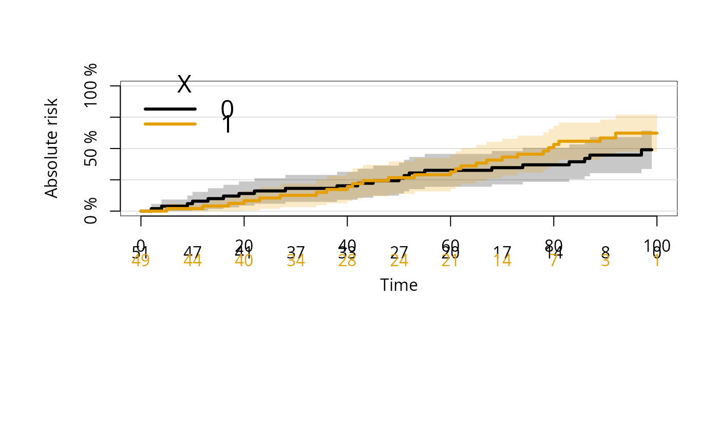
crFit <- prodlim(Hist(time,event)~X,data=CompRiskFrame)
summary(crFit)
#> X time cause n.risk n.event n.lost cuminc se.cuminc lower upper
#> 1 0 1.0 1 51 0 0 0.0000 0.0000 0.0000 0.0000
#> 2 0 25.8 1 39 0 0 0.1611 0.0522 0.0588 0.2634
#> 3 0 50.5 1 26 0 0 0.2634 0.0628 0.1404 0.3864
#> 4 0 75.2 1 15 0 0 0.3697 0.0695 0.2336 0.5058
#> 5 0 100.0 1 0 0 0 NA NA NA NA
#> 6 1 1.0 1 49 0 0 0.0000 0.0000 0.0000 0.0000
#> 7 1 25.8 1 36 0 0 0.1045 0.0443 0.0178 0.1913
#> 8 1 50.5 1 24 0 0 0.2669 0.0663 0.1370 0.3968
#> 9 1 75.2 1 10 0 0 0.4548 0.0752 0.3075 0.6021
#> 10 1 100.0 1 1 0 1 0.6228 0.0755 0.4747 0.7708
#> 11 0 1.0 2 51 0 0 0.0000 0.0000 0.0000 0.0000
#> 12 0 25.8 2 39 0 0 0.0409 0.0283 0.0000 0.0965
#> 13 0 50.5 2 26 0 0 0.2046 0.0577 0.0915 0.3177
#> 14 0 75.2 2 15 0 0 0.2900 0.0654 0.1619 0.4181
#> 15 0 100.0 2 0 0 0 NA NA NA NA
#> 16 1 1.0 2 49 1 0 0.0204 0.0202 0.0000 0.0600
#> 17 1 25.8 2 36 0 0 0.1245 0.0476 0.0312 0.2177
#> 18 1 50.5 2 24 0 0 0.1694 0.0548 0.0621 0.2767
#> 19 1 75.2 2 10 0 0 0.2868 0.0676 0.1543 0.4193
#> 20 1 100.0 2 1 0 1 0.3385 0.0717 0.1979 0.4790
plot(crFit)
##----------continuous covariate: Stone-Beran estimate------------
SB=prodlim(Surv(time,status)~X2,data=dat)
summary(SB,newdata=data.frame(X2=c(-0.3,0,.5)))
#> X2 time n.risk n.event n.lost surv se.surv lower upper
#> 1 -0.3 0.321 17 0 0 1.0000 0.0000 1.0000 1.000
#> 2 -0.3 2.632 13 0 0 0.9286 0.0688 0.7937 1.000
#> 3 -0.3 6.096 8 0 0 0.6190 0.1344 0.3556 0.883
#> 4 -0.3 7.816 3 0 0 0.3316 0.1437 0.0501 0.613
#> 5 -0.3 14.678 1 0 1 0.1658 0.1375 0.0000 0.435
#> 6 0.0 0.321 17 0 0 1.0000 0.0000 1.0000 1.000
#> 7 0.0 2.632 13 0 0 0.9286 0.0688 0.7937 1.000
#> 8 0.0 6.096 8 0 0 0.6190 0.1344 0.3556 0.883
#> 9 0.0 7.816 4 0 0 0.3611 0.1391 0.0885 0.634
#> 10 0.0 14.678 1 0 1 0.1354 0.1158 0.0000 0.362
#> 11 0.5 0.321 16 0 1 1.0000 0.0000 1.0000 1.000
#> 12 0.5 2.632 10 0 0 0.7692 0.1169 0.5402 0.998
#> 13 0.5 6.096 6 0 0 0.4615 0.1383 0.1905 0.733
#> 14 0.5 7.816 3 0 0 0.2885 0.1311 0.0316 0.545
#> 15 0.5 14.678 1 0 1 0.0962 0.0898 0.0000 0.272
##-------------both discrete and continuous covariates------------
prodlim(Surv(time,status)~X2+X1,data=dat)
#>
#> Call: prodlim(formula = Surv(time, status) ~ X2 + X1, data = dat)
#>
#> Stratified Stone-Beran estimator for the conditional event time survival function
#>
#> Discrete predictor variables: X1
#> Continuous predictor variables: X2
#>
#> Right-censored response of a survival model
#>
#> No.Observations: 30
#>
#> Pattern:
#> Freq
#> event 15
#> right.censored 15
##----------------------interval censored data----------------------
dat <- data.frame(L=1:10,R=c(2,3,12,8,9,10,7,12,12,12),status=c(1,1,0,1,1,1,1,0,0,0))
with(dat,Hist(time=list(L,R),event=status))
#>
#> Interval-censored response of a survival model
#>
#> No.Observations: 10
#>
#> Pattern:
#> Freq
#> exact.time 1
#> interval-censored 5
#> right-censored 4
dat$event=1
npmle.fitml <- prodlim(Hist(time=list(L,R),event)~1,data=dat)
##-------------competing risks-------------------
CompRiskFrame <- data.frame(time=1:100,event=rbinom(100,2,.5),X=rbinom(100,1,.5))
crFit <- prodlim(Hist(time,event)~X,data=CompRiskFrame)
summary(crFit)
#> X time cause n.risk n.event n.lost cuminc se.cuminc lower upper
#> 1 0 1.0 1 51 0 0 0.0000 0.0000 0.0000 0.0000
#> 2 0 25.8 1 39 0 0 0.1611 0.0522 0.0588 0.2634
#> 3 0 50.5 1 26 0 0 0.2634 0.0628 0.1404 0.3864
#> 4 0 75.2 1 15 0 0 0.3697 0.0695 0.2336 0.5058
#> 5 0 100.0 1 0 0 0 NA NA NA NA
#> 6 1 1.0 1 49 0 0 0.0000 0.0000 0.0000 0.0000
#> 7 1 25.8 1 36 0 0 0.1045 0.0443 0.0178 0.1913
#> 8 1 50.5 1 24 0 0 0.2669 0.0663 0.1370 0.3968
#> 9 1 75.2 1 10 0 0 0.4548 0.0752 0.3075 0.6021
#> 10 1 100.0 1 1 0 1 0.6228 0.0755 0.4747 0.7708
#> 11 0 1.0 2 51 0 0 0.0000 0.0000 0.0000 0.0000
#> 12 0 25.8 2 39 0 0 0.0409 0.0283 0.0000 0.0965
#> 13 0 50.5 2 26 0 0 0.2046 0.0577 0.0915 0.3177
#> 14 0 75.2 2 15 0 0 0.2900 0.0654 0.1619 0.4181
#> 15 0 100.0 2 0 0 0 NA NA NA NA
#> 16 1 1.0 2 49 1 0 0.0204 0.0202 0.0000 0.0600
#> 17 1 25.8 2 36 0 0 0.1245 0.0476 0.0312 0.2177
#> 18 1 50.5 2 24 0 0 0.1694 0.0548 0.0621 0.2767
#> 19 1 75.2 2 10 0 0 0.2868 0.0676 0.1543 0.4193
#> 20 1 100.0 2 1 0 1 0.3385 0.0717 0.1979 0.4790
plot(crFit)
 summary(crFit,cause=2)
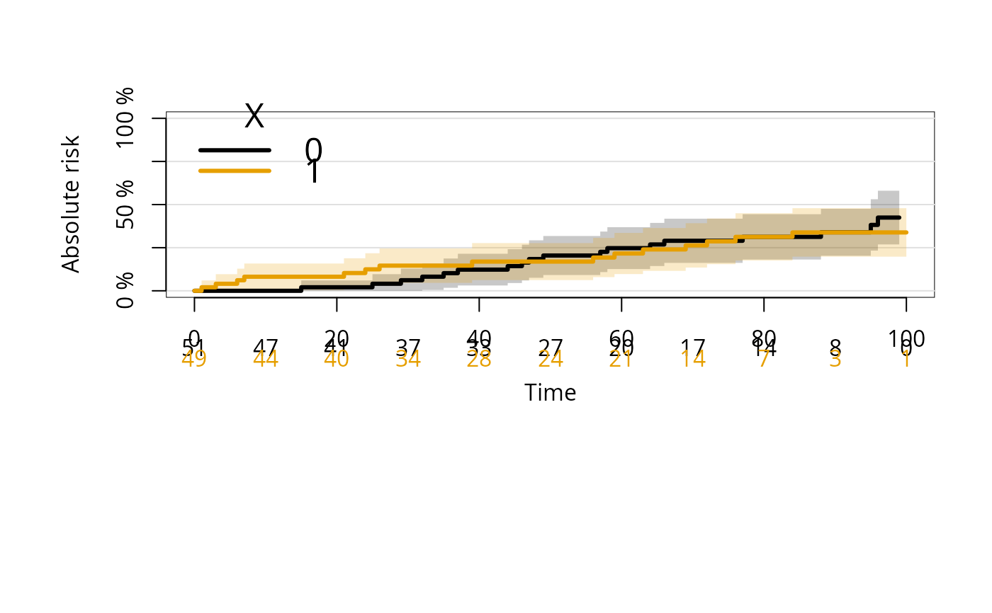
#> X time cause n.risk n.event n.lost cuminc se.cuminc lower upper
#> 1 0 1.0 2 51 0 0 0.0000 0.0000 0.0000 0.0000
#> 2 0 25.8 2 39 0 0 0.0409 0.0283 0.0000 0.0965
#> 3 0 50.5 2 26 0 0 0.2046 0.0577 0.0915 0.3177
#> 4 0 75.2 2 15 0 0 0.2900 0.0654 0.1619 0.4181
#> 5 0 100.0 2 0 0 0 NA NA NA NA
#> 6 1 1.0 2 49 1 0 0.0204 0.0202 0.0000 0.0600
#> 7 1 25.8 2 36 0 0 0.1245 0.0476 0.0312 0.2177
#> 8 1 50.5 2 24 0 0 0.1694 0.0548 0.0621 0.2767
#> 9 1 75.2 2 10 0 0 0.2868 0.0676 0.1543 0.4193
#> 10 1 100.0 2 1 0 1 0.3385 0.0717 0.1979 0.4790
plot(crFit,cause=2)
summary(crFit,cause=2)
#> X time cause n.risk n.event n.lost cuminc se.cuminc lower upper
#> 1 0 1.0 2 51 0 0 0.0000 0.0000 0.0000 0.0000
#> 2 0 25.8 2 39 0 0 0.0409 0.0283 0.0000 0.0965
#> 3 0 50.5 2 26 0 0 0.2046 0.0577 0.0915 0.3177
#> 4 0 75.2 2 15 0 0 0.2900 0.0654 0.1619 0.4181
#> 5 0 100.0 2 0 0 0 NA NA NA NA
#> 6 1 1.0 2 49 1 0 0.0204 0.0202 0.0000 0.0600
#> 7 1 25.8 2 36 0 0 0.1245 0.0476 0.0312 0.2177
#> 8 1 50.5 2 24 0 0 0.1694 0.0548 0.0621 0.2767
#> 9 1 75.2 2 10 0 0 0.2868 0.0676 0.1543 0.4193
#> 10 1 100.0 2 1 0 1 0.3385 0.0717 0.1979 0.4790
plot(crFit,cause=2)
 # Changing the cens.code:
dat <- data.frame(time=1:10,status=c(1,2,1,2,5,5,1,1,2,2))
fit <- prodlim(Hist(time,status)~1,data=dat)
print(fit$model.response)
#>
#> Uncensored response of a competing.risks model
#>
#> No.Observations: 10
#>
#> Pattern:
#>
#> Cause event
#> 1 4
#> 2 4
#> 5 2
#> unknown 0
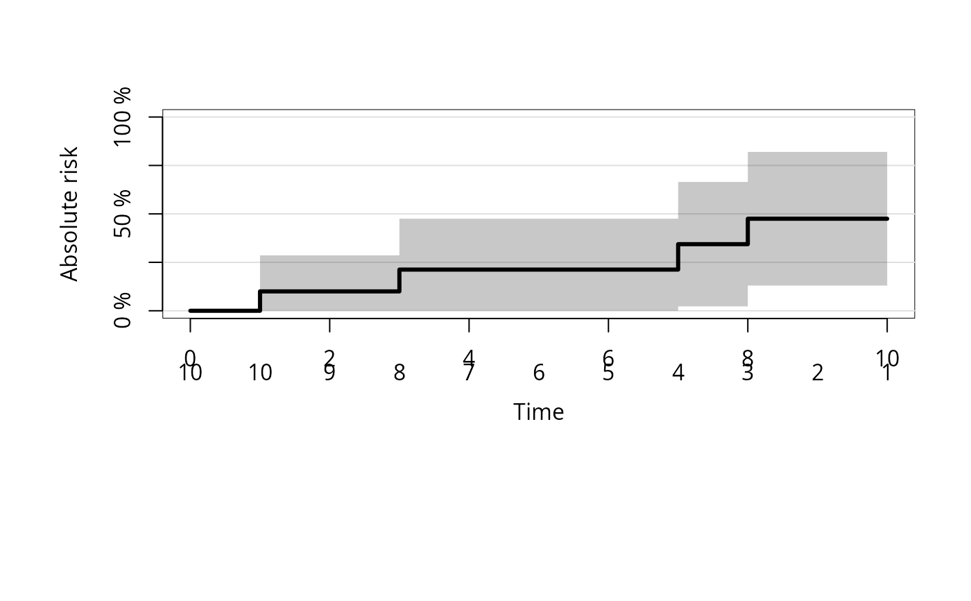
fit <- prodlim(Hist(time,status,cens.code="2")~1,data=dat)
print(fit$model.response)
#>
#> Right-censored response of a competing.risks model
#>
#> No.Observations: 10
#>
#> Pattern:
#>
#> Cause event right.censored
#> 1 4 0
#> 5 2 0
#> unknown 0 4
plot(fit)
# Changing the cens.code:
dat <- data.frame(time=1:10,status=c(1,2,1,2,5,5,1,1,2,2))
fit <- prodlim(Hist(time,status)~1,data=dat)
print(fit$model.response)
#>
#> Uncensored response of a competing.risks model
#>
#> No.Observations: 10
#>
#> Pattern:
#>
#> Cause event
#> 1 4
#> 2 4
#> 5 2
#> unknown 0
fit <- prodlim(Hist(time,status,cens.code="2")~1,data=dat)
print(fit$model.response)
#>
#> Right-censored response of a competing.risks model
#>
#> No.Observations: 10
#>
#> Pattern:
#>
#> Cause event right.censored
#> 1 4 0
#> 5 2 0
#> unknown 0 4
plot(fit)
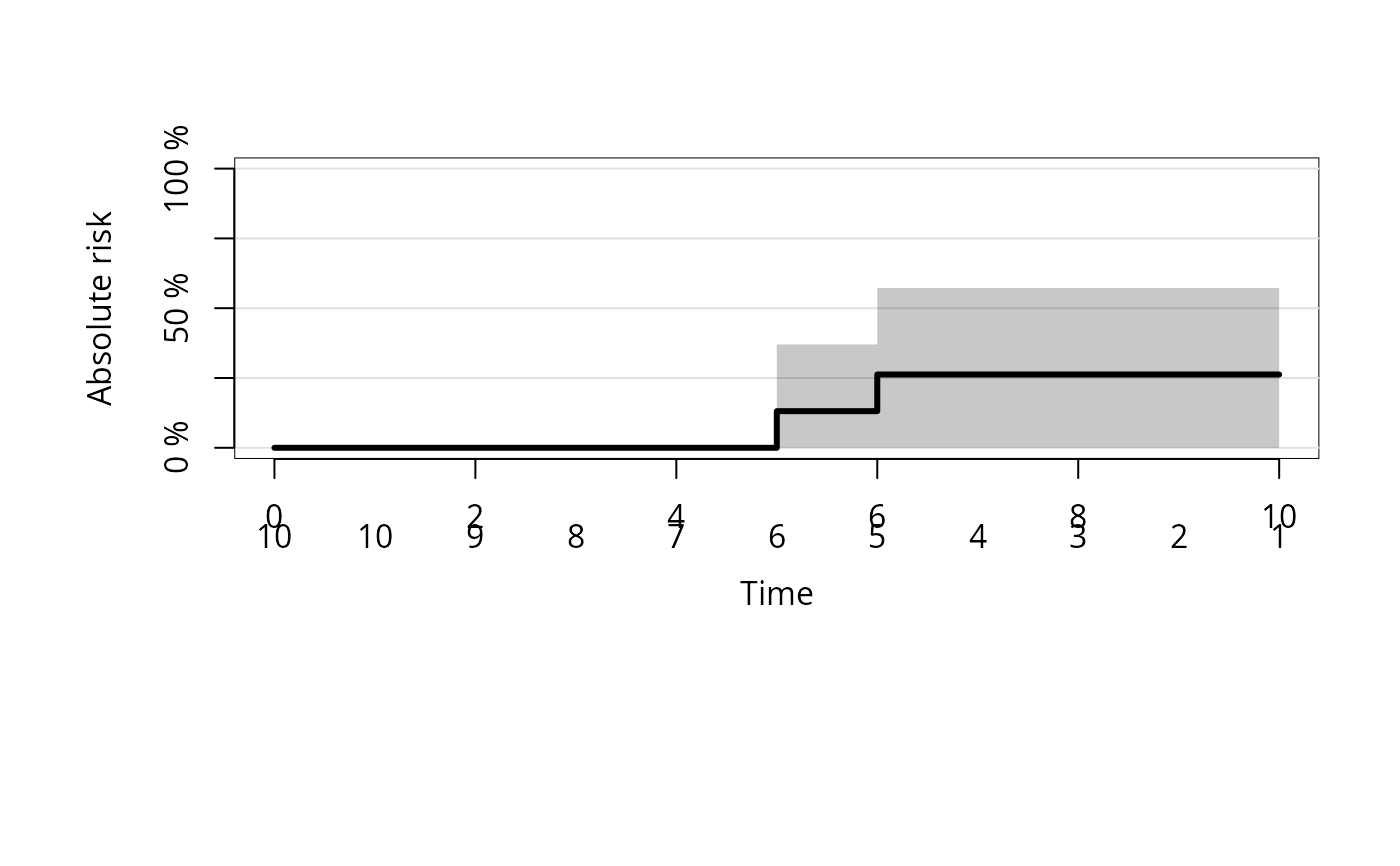
 plot(fit,cause="5")
 ##------------delayed entry----------------------
## left-truncated event times with competing risk endpoint
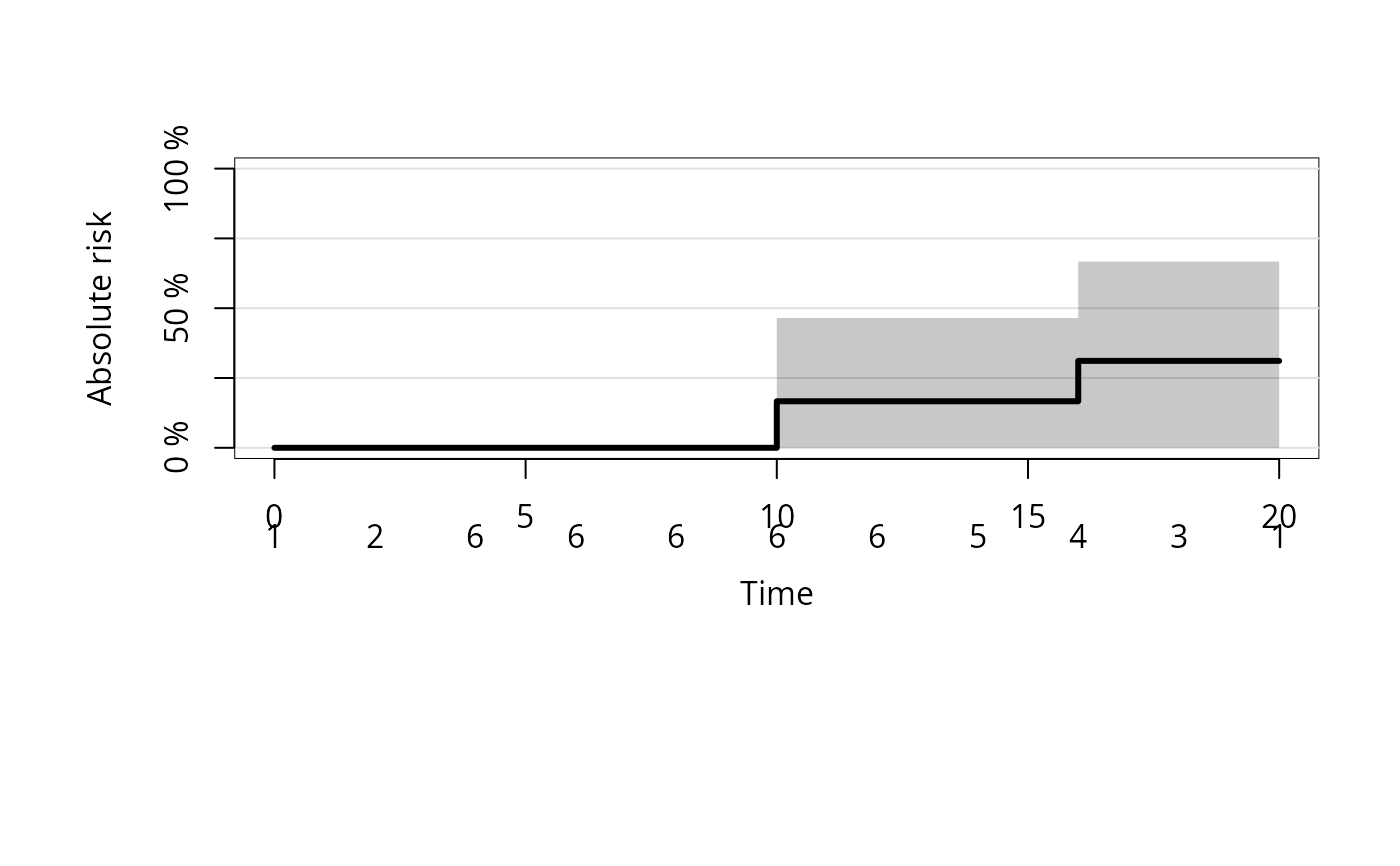
dat <- data.frame(entry=c(7,3,11,12,11,2,1,7,15,17,3),time=10:20,status=c(1,0,2,2,0,0,1,2,0,2,0))
fitd <- prodlim(Hist(time=time,event=status,entry=entry)~1,data=dat)
summary(fitd)
#> time cause n.risk n.event n.lost cuminc se.cuminc lower upper
#> 1 1 1 1 0 0 0.000 0.000 0.0000 0.000
#> 2 2 1 2 0 0 0.000 0.000 0.0000 0.000
#> 3 3 1 4 0 0 0.000 0.000 0.0000 0.000
#> 4 7 1 6 0 0 0.000 0.000 0.0000 0.000
#> 5 10 1 6 1 0 0.167 0.152 0.0000 0.465
#> 6 11 1 5 0 1 0.167 0.152 0.0000 0.465
#> 7 12 1 6 0 0 0.167 0.152 0.0000 0.465
#> 8 13 1 6 0 0 0.167 0.152 0.0000 0.465
#> 9 14 1 5 0 1 0.167 0.152 0.0000 0.465
#> 10 15 1 4 0 1 0.167 0.152 0.0000 0.465
#> 11 16 1 4 1 0 0.311 0.181 0.0000 0.667
#> 12 17 1 3 0 0 0.311 0.181 0.0000 0.667
#> 13 18 1 3 0 1 0.311 0.181 0.0000 0.667
#> 14 19 1 2 0 0 0.311 0.181 0.0000 0.667
#> 15 20 1 1 0 1 0.311 0.181 0.0000 0.667
#> 16 1 2 1 0 0 0.000 0.000 0.0000 0.000
#> 17 2 2 2 0 0 0.000 0.000 0.0000 0.000
#> 18 3 2 4 0 0 0.000 0.000 0.0000 0.000
#> 19 7 2 6 0 0 0.000 0.000 0.0000 0.000
#> 20 10 2 6 0 0 0.000 0.000 0.0000 0.000
#> 21 11 2 5 0 1 0.000 0.000 0.0000 0.000
#> 22 12 2 6 1 0 0.139 0.129 0.0000 0.392
#> 23 13 2 6 1 0 0.255 0.156 0.0000 0.561
#> 24 14 2 5 0 1 0.255 0.156 0.0000 0.561
#> 25 15 2 4 0 1 0.255 0.156 0.0000 0.561
#> 26 16 2 4 0 0 0.255 0.156 0.0000 0.561
#> 27 17 2 3 1 0 0.399 0.183 0.0402 0.758
#> 28 18 2 3 0 1 0.399 0.183 0.0402 0.758
#> 29 19 2 2 1 0 0.544 0.191 0.1702 0.918
#> 30 20 2 1 0 1 0.544 0.191 0.1702 0.918
plot(fitd)
##------------delayed entry----------------------
## left-truncated event times with competing risk endpoint
dat <- data.frame(entry=c(7,3,11,12,11,2,1,7,15,17,3),time=10:20,status=c(1,0,2,2,0,0,1,2,0,2,0))
fitd <- prodlim(Hist(time=time,event=status,entry=entry)~1,data=dat)
summary(fitd)
#> time cause n.risk n.event n.lost cuminc se.cuminc lower upper
#> 1 1 1 1 0 0 0.000 0.000 0.0000 0.000
#> 2 2 1 2 0 0 0.000 0.000 0.0000 0.000
#> 3 3 1 4 0 0 0.000 0.000 0.0000 0.000
#> 4 7 1 6 0 0 0.000 0.000 0.0000 0.000
#> 5 10 1 6 1 0 0.167 0.152 0.0000 0.465
#> 6 11 1 5 0 1 0.167 0.152 0.0000 0.465
#> 7 12 1 6 0 0 0.167 0.152 0.0000 0.465
#> 8 13 1 6 0 0 0.167 0.152 0.0000 0.465
#> 9 14 1 5 0 1 0.167 0.152 0.0000 0.465
#> 10 15 1 4 0 1 0.167 0.152 0.0000 0.465
#> 11 16 1 4 1 0 0.311 0.181 0.0000 0.667
#> 12 17 1 3 0 0 0.311 0.181 0.0000 0.667
#> 13 18 1 3 0 1 0.311 0.181 0.0000 0.667
#> 14 19 1 2 0 0 0.311 0.181 0.0000 0.667
#> 15 20 1 1 0 1 0.311 0.181 0.0000 0.667
#> 16 1 2 1 0 0 0.000 0.000 0.0000 0.000
#> 17 2 2 2 0 0 0.000 0.000 0.0000 0.000
#> 18 3 2 4 0 0 0.000 0.000 0.0000 0.000
#> 19 7 2 6 0 0 0.000 0.000 0.0000 0.000
#> 20 10 2 6 0 0 0.000 0.000 0.0000 0.000
#> 21 11 2 5 0 1 0.000 0.000 0.0000 0.000
#> 22 12 2 6 1 0 0.139 0.129 0.0000 0.392
#> 23 13 2 6 1 0 0.255 0.156 0.0000 0.561
#> 24 14 2 5 0 1 0.255 0.156 0.0000 0.561
#> 25 15 2 4 0 1 0.255 0.156 0.0000 0.561
#> 26 16 2 4 0 0 0.255 0.156 0.0000 0.561
#> 27 17 2 3 1 0 0.399 0.183 0.0402 0.758
#> 28 18 2 3 0 1 0.399 0.183 0.0402 0.758
#> 29 19 2 2 1 0 0.544 0.191 0.1702 0.918
#> 30 20 2 1 0 1 0.544 0.191 0.1702 0.918
plot(fitd)