Visualize Fitted Log-linear Models
plot.loglm.RdVisualize fitted "loglm" objects by mosaic or
association plots.
Arguments
- x
a fitted
"loglm"object, seeloglm.- panel
a panel function for visualizing the observed values, residuals and expected values. Currently,
mosaicandassocin vcd.- type
a character string indicating whether the observed or the expected values of the table should be visualized.
- residuals_type
a character string indicating the type of residuals to be computed.
- gp
object of class
"gpar", shading function or a corresponding generating function (see details andshadings). Ignored ifshade = FALSE.- gp_args
list of arguments for the shading-generating function, if specified.
- ...
Other arguments passed to the
panelfunction.
Details
The plot method for "loglm" objects by default visualizes
the model using a mosaic plot (can be changed to an association plot
by setting panel = assoc) with a shading based on the residuals
of this model. The legend also reports the corresponding p value of the
associated goodness-of-fit test. The mosaic and assoc methods
are simple convenience interfaces to this plot method, setting
the panel argument accordingly.
Value
The "structable" visualized is returned invisibly.
Examples
library(MASS)
## mosaic display for PreSex model
data("PreSex")
fm <- loglm(~ PremaritalSex * ExtramaritalSex * (Gender + MaritalStatus),
data = aperm(PreSex, c(3, 2, 4, 1)))
fm
#> Call:
#> loglm(formula = ~PremaritalSex * ExtramaritalSex * (Gender +
#> MaritalStatus), data = aperm(PreSex, c(3, 2, 4, 1)))
#>
#> Statistics:
#> X^2 df P(> X^2)
#> Likelihood Ratio 5.245519 4 0.2630205
#> Pearson 5.238526 4 0.2636870
## visualize Pearson statistic
plot(fm, split_vertical = TRUE)
 ## visualize LR statistic
plot(fm, split_vertical = TRUE, residuals_type = "deviance")
## visualize LR statistic
plot(fm, split_vertical = TRUE, residuals_type = "deviance")
 ## conditional independence in UCB admissions data
data("UCBAdmissions")
fm <- loglm(~ Dept * (Gender + Admit), data = aperm(UCBAdmissions))
## use mosaic display
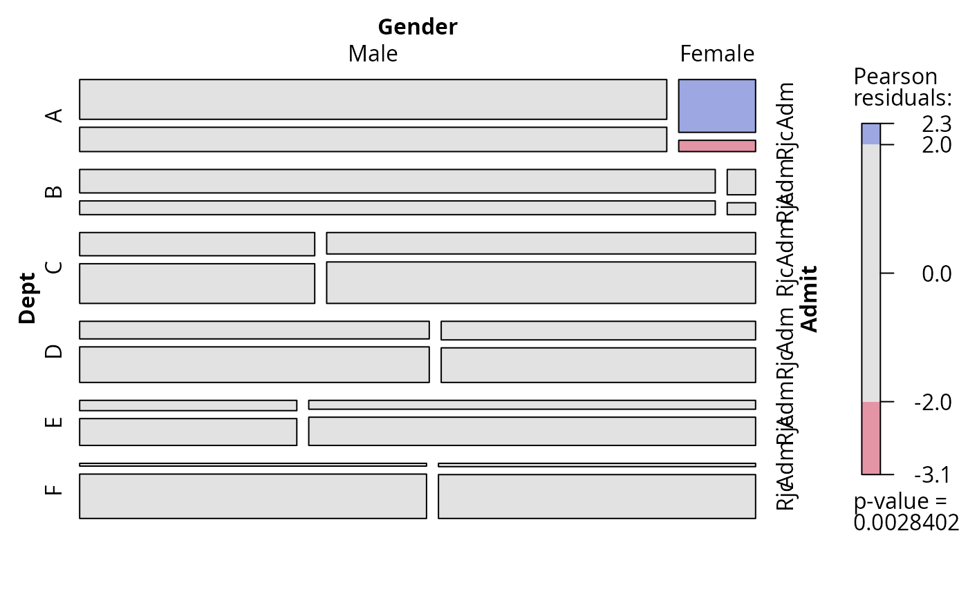
plot(fm, labeling_args = list(abbreviate_labs = c(Admit = 3)))
## conditional independence in UCB admissions data
data("UCBAdmissions")
fm <- loglm(~ Dept * (Gender + Admit), data = aperm(UCBAdmissions))
## use mosaic display
plot(fm, labeling_args = list(abbreviate_labs = c(Admit = 3)))
 ## and association plot
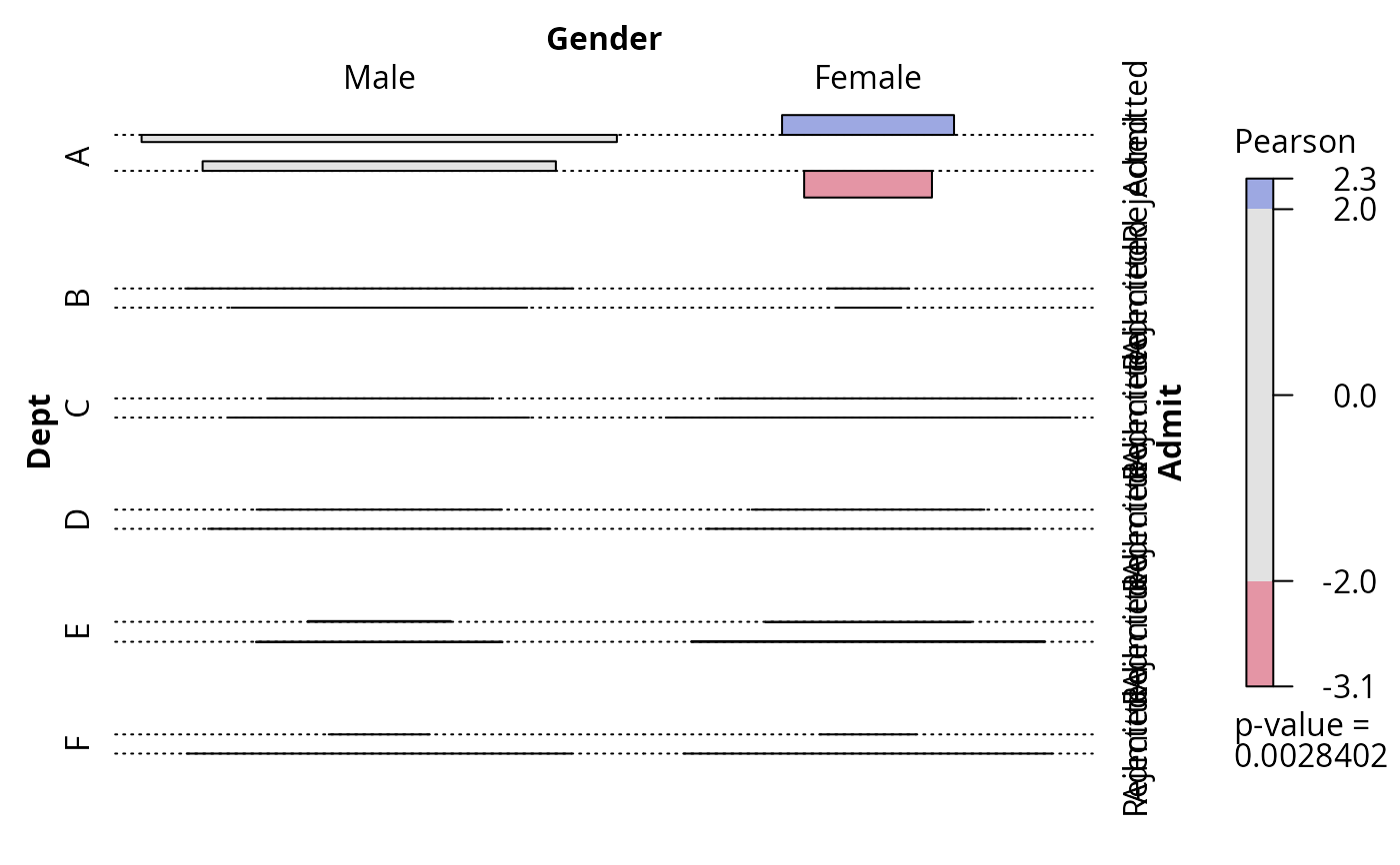
plot(fm, panel = assoc)
## and association plot
plot(fm, panel = assoc)
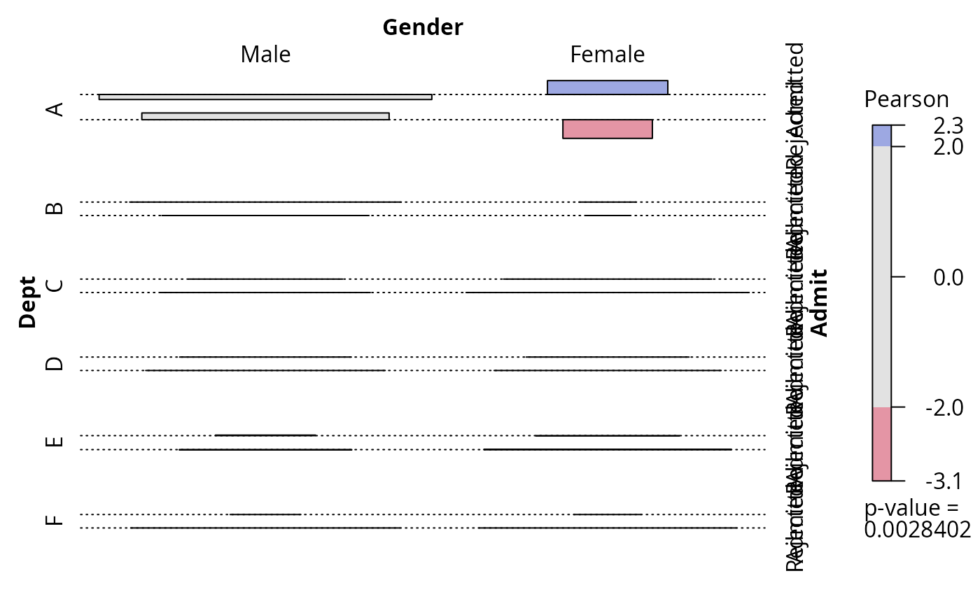 assoc(fm)