This function creates synthetic dataset with various problems such as overdispersion, zero-inflation, etc.
Usage
createData(sampleSize = 100, intercept = 0, fixedEffects = 1,
  quadraticFixedEffects = NULL, numGroups = 10, randomEffectVariance = 1,
  overdispersion = 0, family = poisson(), scale = 1, cor = 0,
  roundPoissonVariance = NULL, pZeroInflation = 0, binomialTrials = 1,
  temporalAutocorrelation = 0, spatialAutocorrelation = 0,
  factorResponse = FALSE, replicates = 1, hasNA = FALSE)
Arguments
- sampleSize
sample size of the dataset.
- intercept
intercept (linear scale).
- fixedEffects
vector of fixed effects (linear scale).
- quadraticFixedEffects
vector of quadratic fixed effects (linear scale).
- numGroups
number of groups for the random effect.
- randomEffectVariance
variance of the random effect (intercept).
- overdispersion
if this is a numeric value, it will be used as the sd of a random normal variate that is added to the linear predictor. Alternatively, a random function can be provided that takes as input the linear predictor.
- family
a family function for the error distribution and link function to be used in the model to simulate data from. (See
stats::family()for details of family functions for GLMs.)- scale
scale if the distribution has a scale (e.g. sd for the Gaussian).
- cor
correlation between predictors.
- roundPoissonVariance
if set, this creates a uniform noise on the Poisson response. The aim of this is to create heteroscedasticity.
- pZeroInflation
probability to set any data point to zero.
- binomialTrials
number of trials for the binomial. Only active if family == binomial.
- temporalAutocorrelation
strength of temporal autocorrelation.
- spatialAutocorrelation
strength of spatial autocorrelation.
- factorResponse
should the response be transformed to a factor (intended to be used for 0/1 data).
- replicates
number of datasets to create.
- hasNA
should an NA be added to the environmental predictor (for test purposes).
Examples
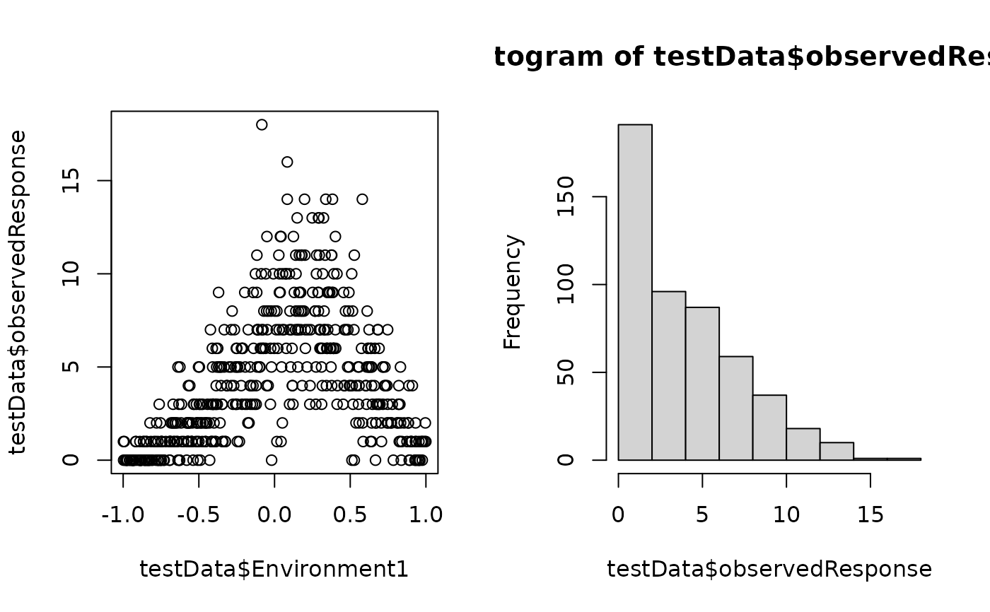
testData = createData(sampleSize = 500, intercept = 2, fixedEffects = c(1),
overdispersion = 0, family = poisson(), quadraticFixedEffects = c(-3),
randomEffectVariance = 0)
par(mfrow = c(1,2))
plot(testData$Environment1, testData$observedResponse)
hist(testData$observedResponse)
 # with zero-inflation
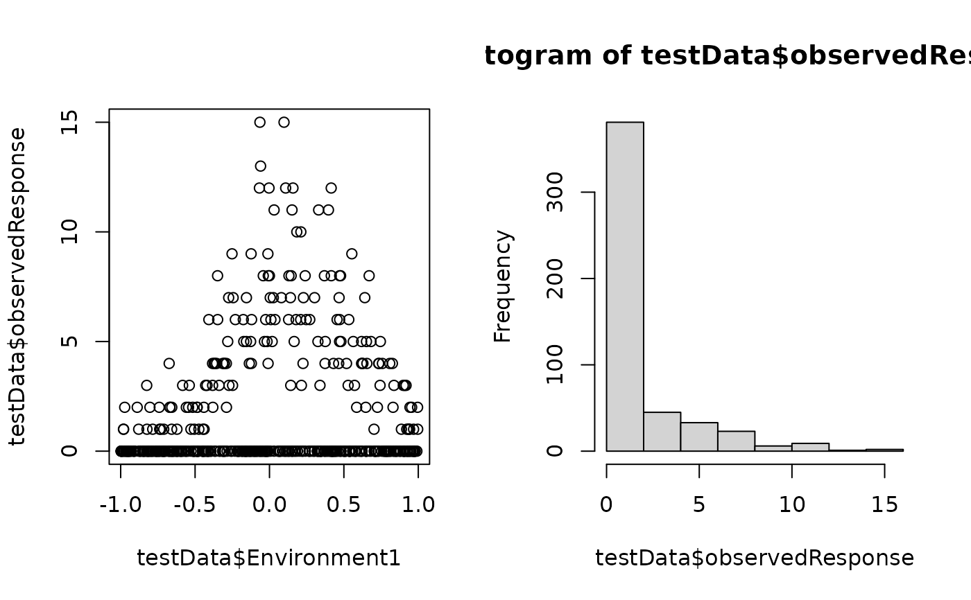
testData = createData(sampleSize = 500, intercept = 2, fixedEffects = c(1),
overdispersion = 0, family = poisson(), quadraticFixedEffects = c(-3),
randomEffectVariance = 0, pZeroInflation = 0.6)
par(mfrow = c(1,2))
plot(testData$Environment1, testData$observedResponse)
hist(testData$observedResponse)
# with zero-inflation
testData = createData(sampleSize = 500, intercept = 2, fixedEffects = c(1),
overdispersion = 0, family = poisson(), quadraticFixedEffects = c(-3),
randomEffectVariance = 0, pZeroInflation = 0.6)
par(mfrow = c(1,2))
plot(testData$Environment1, testData$observedResponse)
hist(testData$observedResponse)
 # binomial with multiple trials
testData = createData(sampleSize = 40, intercept = 2, fixedEffects = c(1),
overdispersion = 0, family = binomial(), quadraticFixedEffects = c(-3),
randomEffectVariance = 0, binomialTrials = 20)
plot(observedResponse1 / observedResponse0 ~ Environment1, data = testData, ylab = "Proportion 1")
# spatial / temporal correlation
testData = createData(sampleSize = 100, family = poisson(), spatialAutocorrelation = 3,
temporalAutocorrelation = 3)
plot(log(observedResponse) ~ time, data = testData)
# binomial with multiple trials
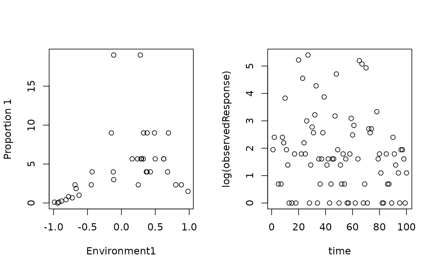
testData = createData(sampleSize = 40, intercept = 2, fixedEffects = c(1),
overdispersion = 0, family = binomial(), quadraticFixedEffects = c(-3),
randomEffectVariance = 0, binomialTrials = 20)
plot(observedResponse1 / observedResponse0 ~ Environment1, data = testData, ylab = "Proportion 1")
# spatial / temporal correlation
testData = createData(sampleSize = 100, family = poisson(), spatialAutocorrelation = 3,
temporalAutocorrelation = 3)
plot(log(observedResponse) ~ time, data = testData)
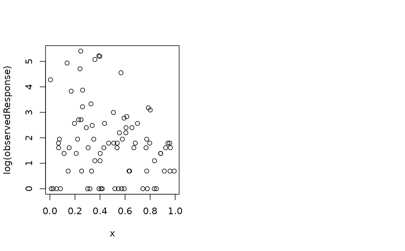
 plot(log(observedResponse) ~ x, data = testData)