Rolling Periods Summary: Statistics and Stylized Facts

A table of estimates of rolling period return measures

Usage

table.RollingPeriods(
  R,
  periods = subset(c(12, 36, 60), c(12, 36, 60) < length(as.matrix(R[, 1]))),
  FUNCS = c("mean", "sd"),
  funcs.names = c("Average", "Std Dev"),
  digits = 4,
  ...
)

table.TrailingPeriodsRel(
  R,
  Rb,
  periods = subset(c(12, 36, 60), c(12, 36, 60) < length(as.matrix(R[, 1]))),
  FUNCS = c("cor", "CAPM.beta"),
  funcs.names = c("Correlation", "Beta"),
  digits = 4,
  ...
)

Arguments

R

an xts, vector, matrix, data frame, timeSeries or zoo object of asset returns

periods

number of periods to use as rolling window(s), subset of c(3, 6, 9, 12, 18, 24, 36, 48)

FUNCS

list of functions to apply the rolling period to

funcs.names

vector of function names used for labeling table rows

digits

number of digits to round results to

...

any other passthru parameters for functions specified in FUNCS

Rb

an xts, vector, matrix, data frame, timeSeries or zoo object of index, benchmark, portfolio, or secondary asset returns to compare against

Details

table.RollingPeriods and table.TrailingPeriods (which are aliases) calculate statistics over rolling windows for individual assets. They apply the FUNCS directly to each column of R independently.

table.TrailingPeriodsRel calculates statistics over rolling windows relative to a benchmark. It applies the FUNCS to each column of R and the corresponding column of Rb simultaneously. This is ideal for relative metrics like CAPM.beta, cor, or tracking error. If you need to calculate metrics requiring a benchmark, use table.TrailingPeriodsRel.

See also

rollapply

Author

Peter Carl

Examples

data(edhec)

# Example 1: Univariate Rolling Statistics
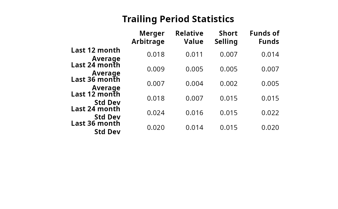
table.TrailingPeriods(edhec[, 10:13], periods = c(12, 24, 36))
#>                       Merger Arbitrage Relative Value Short Selling
#> Last 12 month Average           0.0175         0.0110        0.0074
#> Last 24 month Average           0.0085         0.0055        0.0055
#> Last 36 month Average           0.0069         0.0039        0.0016
#> Last 12 month Std Dev           0.0181         0.0066        0.0154
#> Last 24 month Std Dev           0.0245         0.0164        0.0147
#> Last 36 month Std Dev           0.0203         0.0141        0.0154
#>                       Funds of Funds
#> Last 12 month Average         0.0142
#> Last 24 month Average         0.0074
#> Last 36 month Average         0.0046
#> Last 12 month Std Dev         0.0150
#> Last 24 month Std Dev         0.0217
#> Last 36 month Std Dev         0.0195

# Example 2: Relative Rolling Statistics against a Benchmark
table.TrailingPeriodsRel(edhec[, 10:12],
  Rb = edhec[, 13],
  periods = c(12, 24, 36),
  FUNCS = c("cor", "CAPM.beta"),
  funcs.names = c("Correlation", "Beta")
)
#>                                             Merger Arbitrage Relative Value
#> Last 12 month Correlation to Funds of Funds           0.5337         0.8250
#> Last 24 month Correlation to Funds of Funds           0.8547         0.9427
#> Last 36 month Correlation to Funds of Funds           0.8257         0.9423
#> Last 12 month Beta to Funds of Funds                  0.6456         0.3630
#> Last 24 month Beta to Funds of Funds                  0.9624         0.7103
#> Last 36 month Beta to Funds of Funds                  0.8615         0.6840
#>                                             Short Selling
#> Last 12 month Correlation to Funds of Funds        0.1892
#> Last 24 month Correlation to Funds of Funds       -0.3029
#> Last 36 month Correlation to Funds of Funds       -0.2859
#> Last 12 month Beta to Funds of Funds               0.1946
#> Last 24 month Beta to Funds of Funds              -0.2046
#> Last 36 month Beta to Funds of Funds              -0.2260

result <- table.TrailingPeriods(edhec[, 10:13], periods = c(12, 24, 36))

# \donttest{
# don't test on CRAN, since it requires Suggested packages

require("Hmisc")
textplot(
  format.df(result,
    na.blank = TRUE, numeric.dollar = FALSE,
    cdec = rep(3, dim(result)[2])
  ),
  rmar = 0.8, cmar = 1.5,
  max.cex = .9, halign = "center", valign = "top", row.valign = "center",
  wrap.rownames = 15, wrap.colnames = 10, mar = c(0, 0, 3, 0) + 0.1
)
title(main = "Trailing Period Statistics")

# }