Publication-ready correlation plots

This is a gallery of finished figures — each with the code that produces it — for the kinds of correlograms that show up in papers. For the argument-by-argument tour of every option, see vignette("ggcorrplot").

Two facts make ggcorrplot well suited to publication work: it takes a correlation matrix you already have (so it never gets between you and your statistics), and it returns a plain ggplot object, so any figure here can be restyled, titled, and combined with +.

library(ggcorrplot)
library(ggplot2)

data(mtcars)
corr <- round(cor(mtcars), 1)
p.mat <- cor_pmat(mtcars)

The clustered correlogram

The workhorse figure: reorder the variables by hierarchical clustering so correlated variables sit together and the block structure is visible, and draw thin white separators between cells.

ggcorrplot(corr, hc.order = TRUE, outline.color = "white")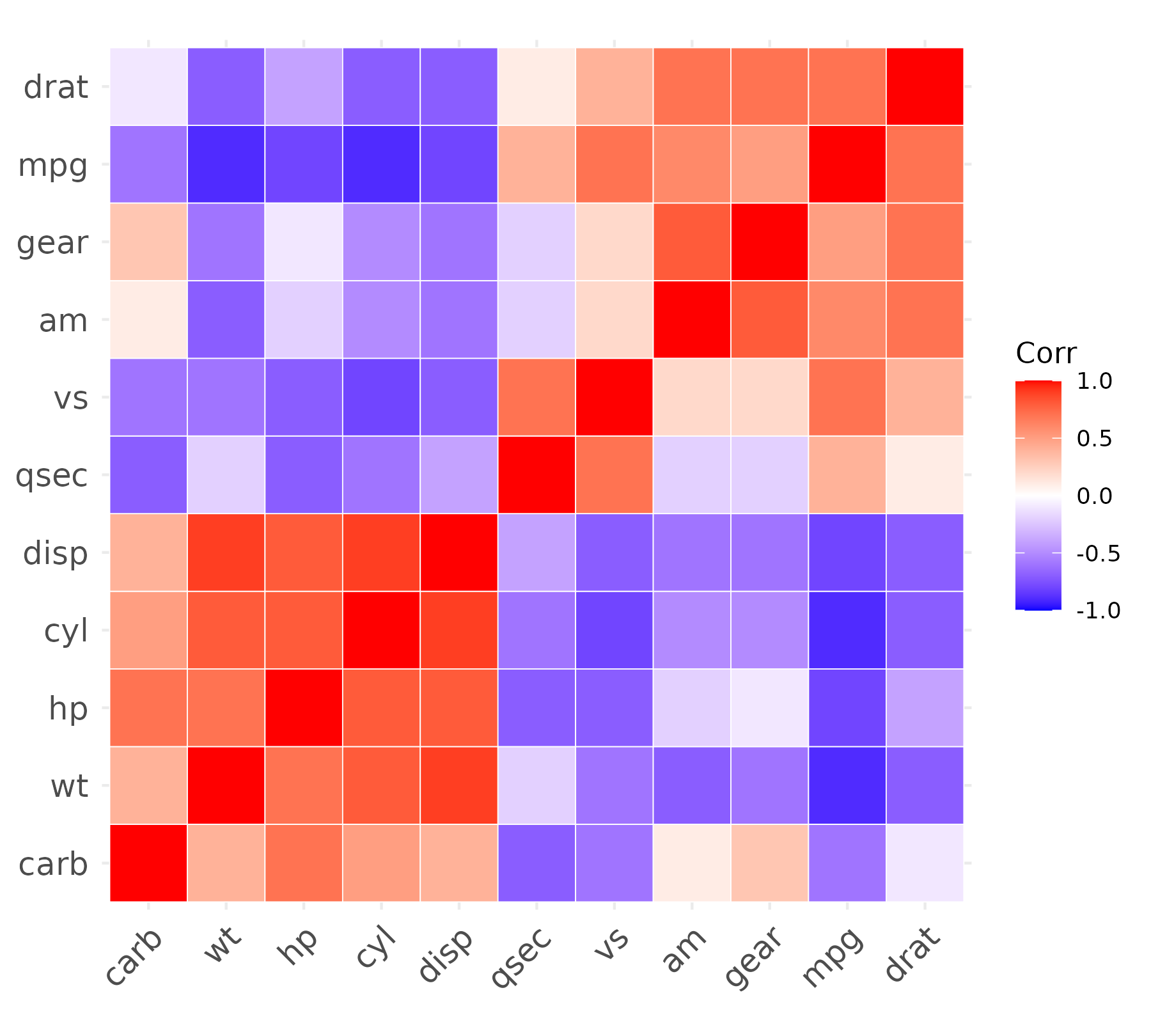

Lower triangle with coefficients

For a symmetric matrix the two triangles are redundant, so a paper usually shows one, often with the coefficients printed in the cells — a figure that replaces a correlation table.

ggcorrplot(corr, hc.order = TRUE, type = "lower", lab = TRUE, lab_size = 3)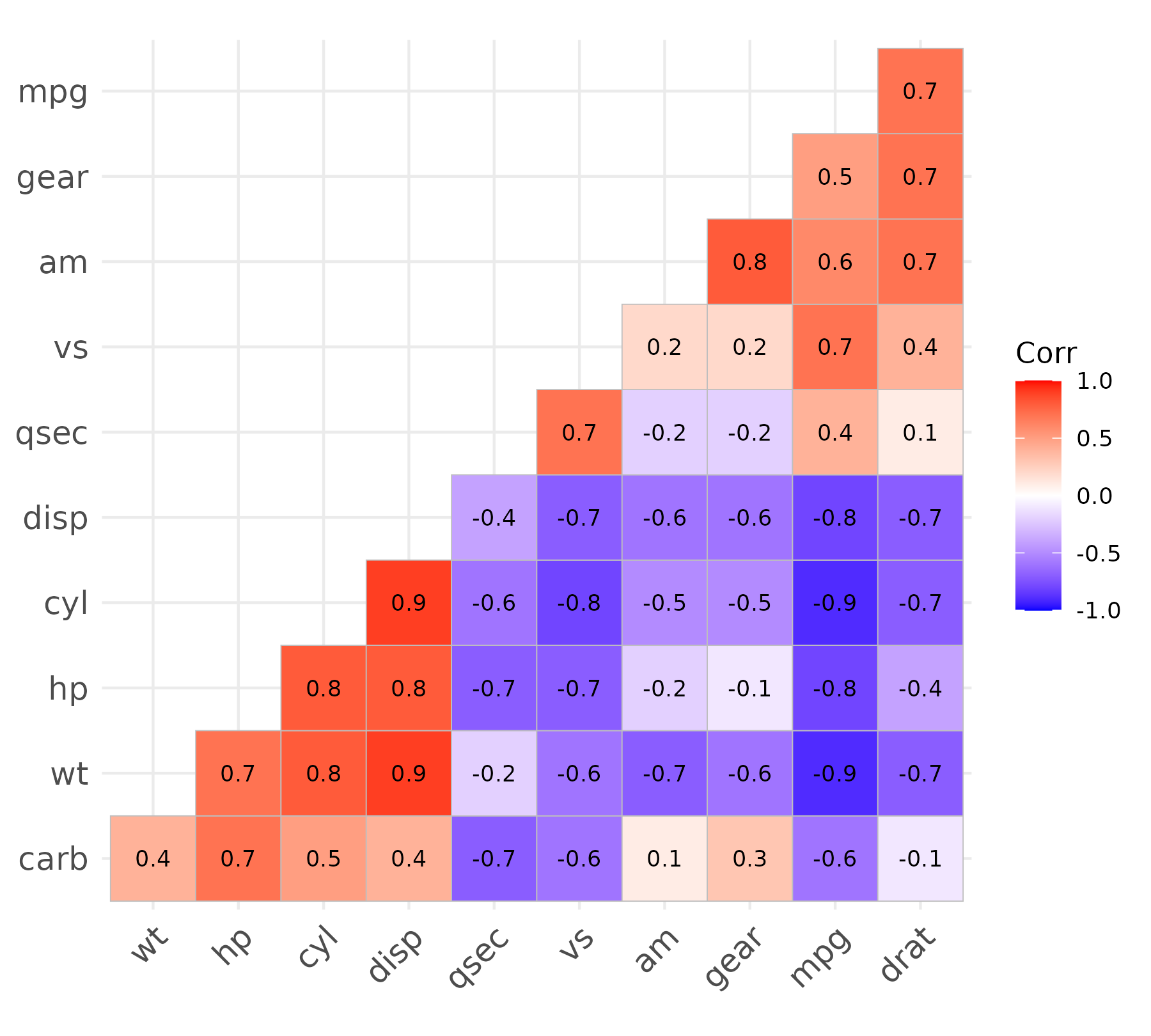

Marking significance

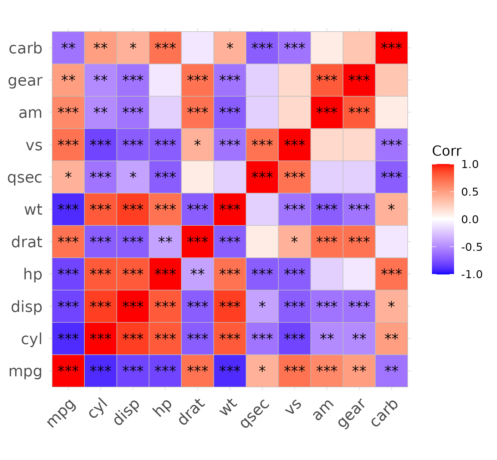
Supply the p-value matrix from cor_pmat() and choose how to convey significance. insig = "blank" drops the non-significant cells; insig = "stars" instead marks the significant ones with */**/*** — a standalone significance map.

# non-significant cells left blank
ggcorrplot(corr, hc.order = TRUE, type = "lower", p.mat = p.mat, insig = "blank")
# significant cells starred
ggcorrplot(corr, p.mat = p.mat, insig = "stars")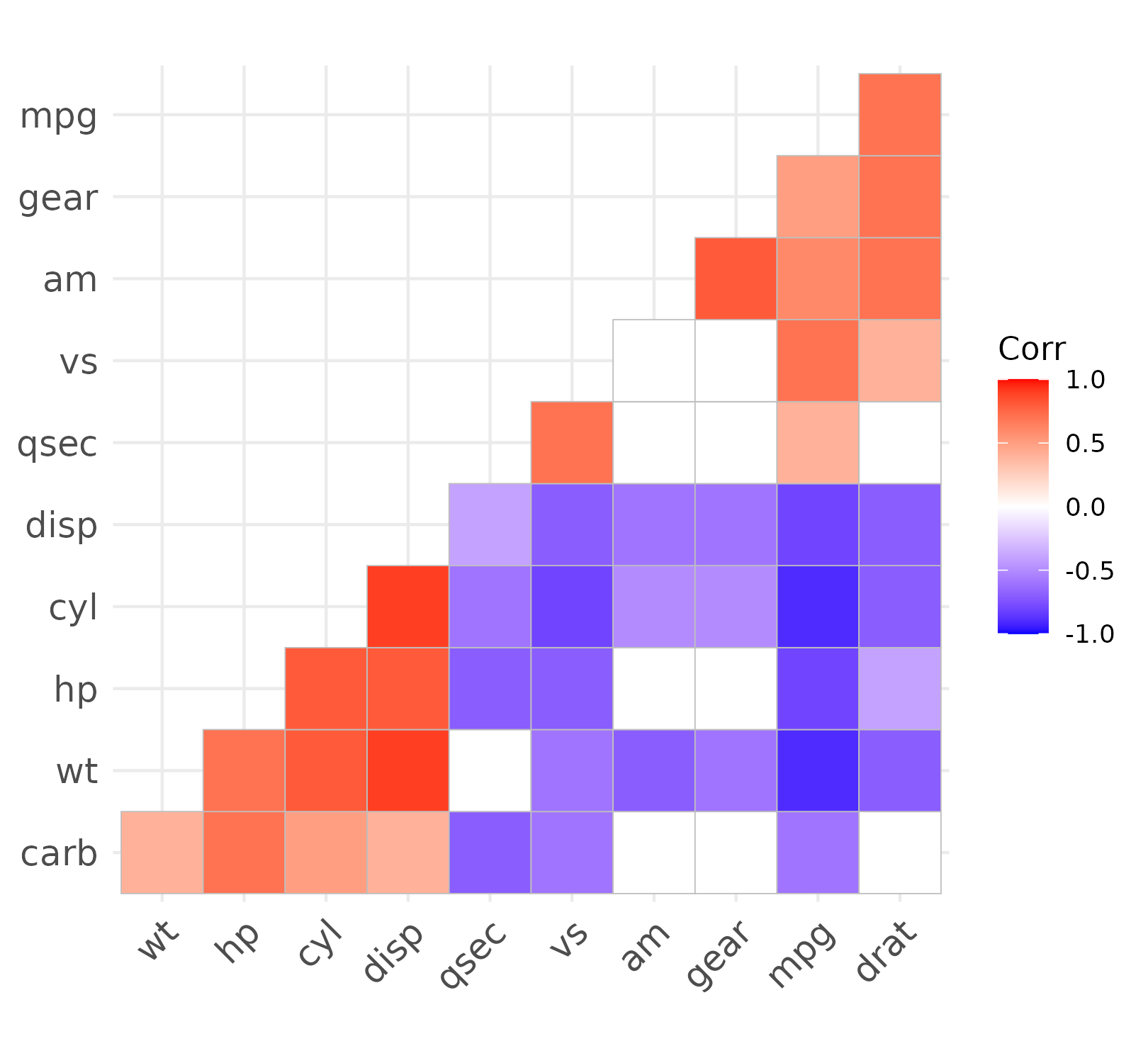

The default, insig = "pch", crosses out the non-significant cells with an X instead.

Circles for magnitude

method = "circle" encodes the correlation with the circle’s area, so strong correlations pop out — the familiar corrplot look, drawn in ggplot2.

ggcorrplot(corr, method = "circle", hc.order = TRUE, type = "upper", outline.color = "white")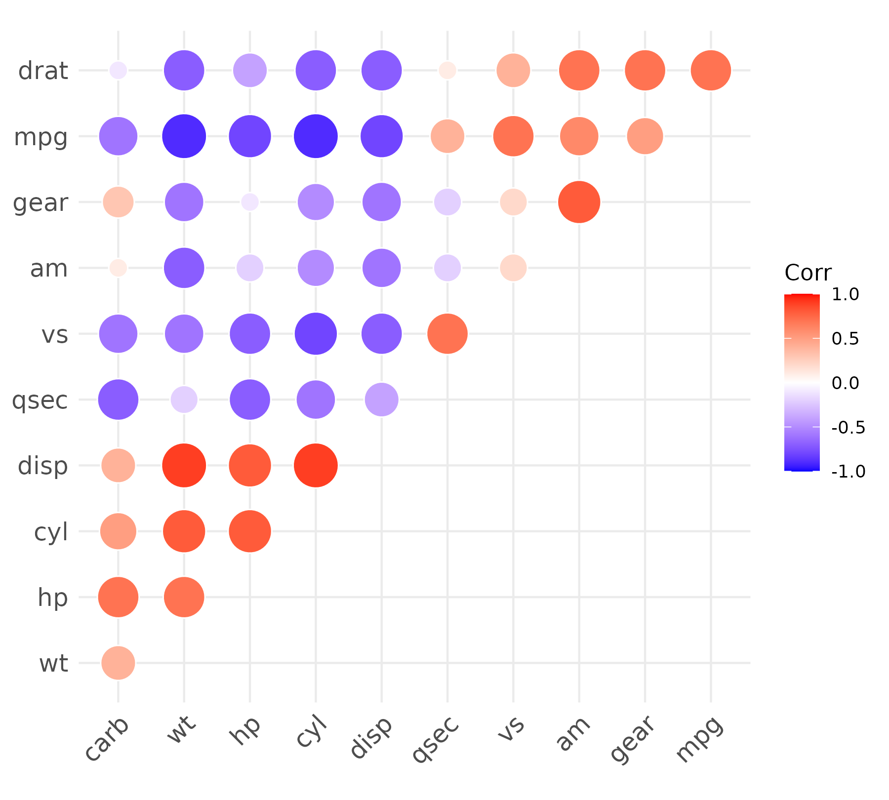

Size-scaled squares

scale.square = TRUE sizes the squares by the absolute correlation, so magnitude is encoded by both area and color at once — the classic corrplot square look. Near-zero cells shrink to small squares while the strong correlations dominate, which reads well for large matrices and for colorblind viewers.

ggcorrplot(corr, scale.square = TRUE, hc.order = TRUE, outline.color = "white")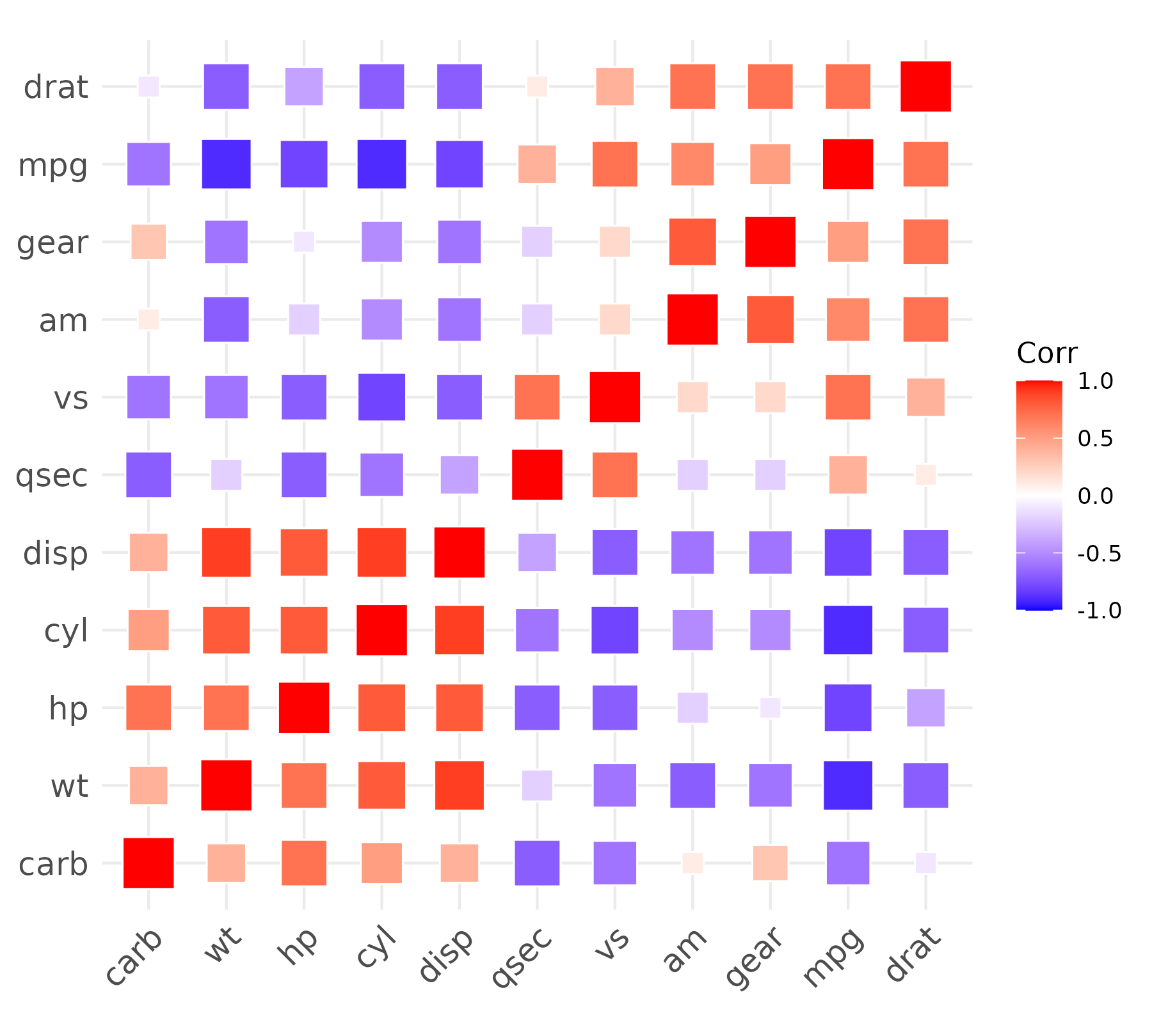

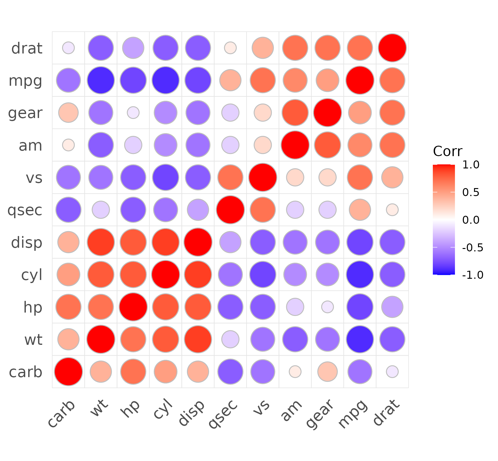
corrplot-style boxed cells

cell.grid = TRUE draws a light rectangle around every cell and drops the gridlines that otherwise run through the glyph centers, so each sized glyph sits inside its own box. Combined with scale.square = TRUE (or method = "circle") this is the boxed-cell corrplot signature, drawn in ggplot2. It has no effect on a plain full-tile square heatmap, whose cells already have a border.

# size-scaled squares in boxed cells
ggcorrplot(corr, scale.square = TRUE, cell.grid = TRUE, hc.order = TRUE, outline.color = "white")
# circles in boxed cells
ggcorrplot(corr, method = "circle", cell.grid = TRUE, hc.order = TRUE)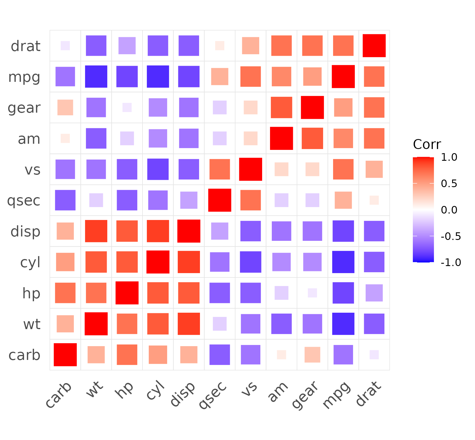

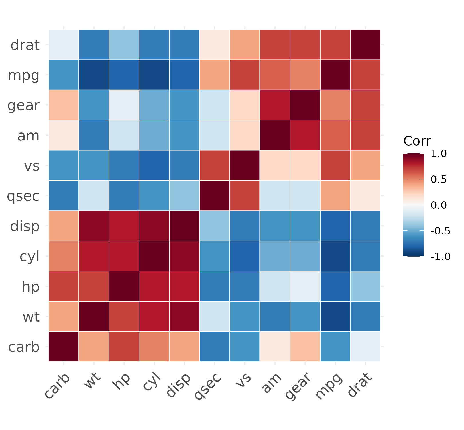
A colorblind-safe palette

preset = "publication" is a one-token beautiful default (white separators + the colorblind-safe RdBu palette). For a specific journal look, set colors and ggtheme yourself.

# one-token publication preset
ggcorrplot(corr, hc.order = TRUE, preset = "publication")
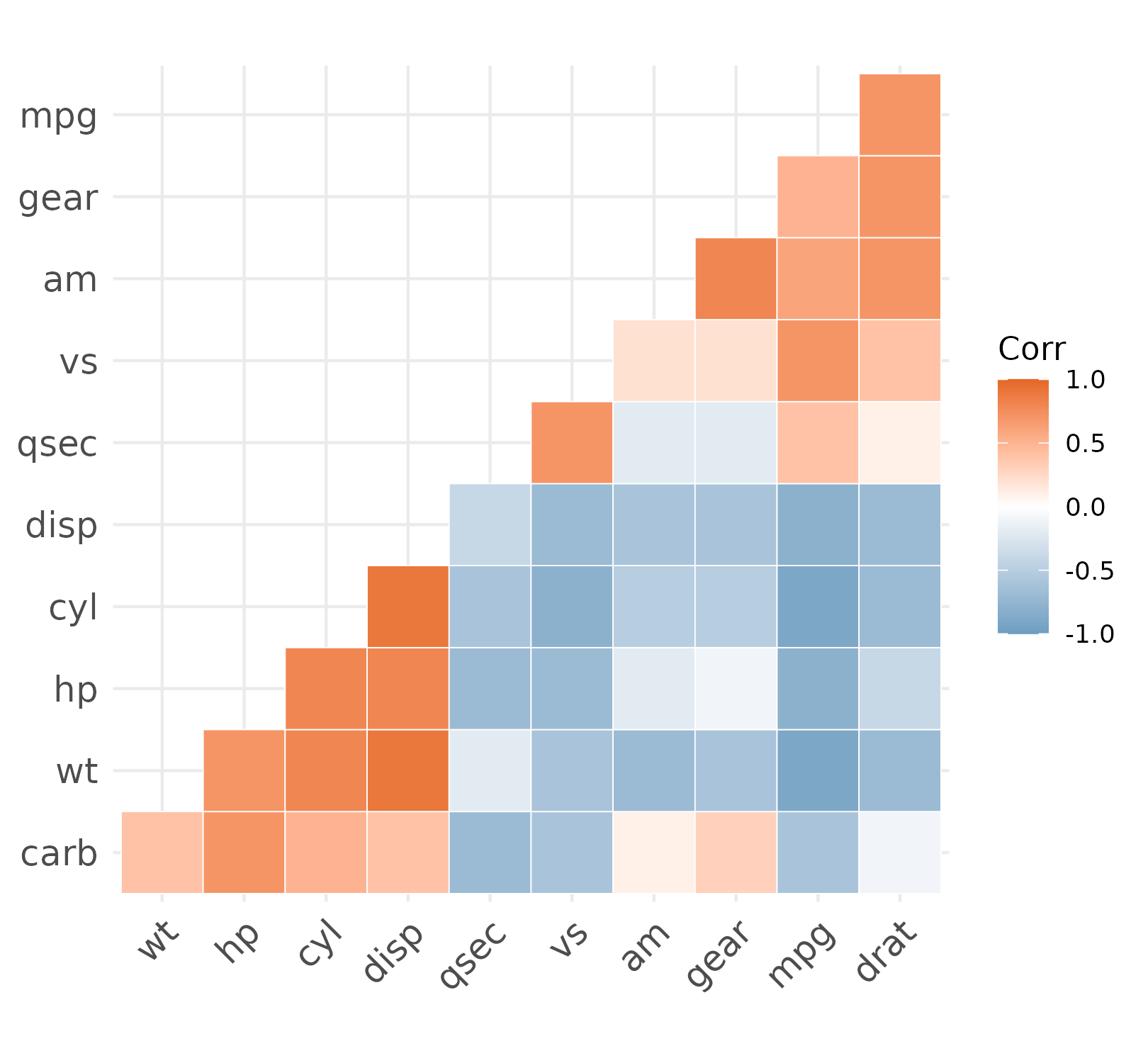
# a custom diverging palette on a minimal theme
ggcorrplot(corr,
  hc.order = TRUE, type = "lower", outline.color = "white",
  ggtheme = theme_minimal, colors = c("#6D9EC1", "white", "#E46726")
)

A clean, edgeless heatmap

A correlogram of solid colored squares with no cell border — the look used in many module–trait and omics papers. method = "square" is a full-tile heatmap; outline.color = NA removes the border. Reverse the default gradient to c("red", "white", "blue") for red-negative / blue-positive, and put the variable names on top with a one-line scale.

ggcorrplot(corr,
  outline.color = NA,
  colors = c("red", "white", "blue"),
  legend.title = "Correlation"
) +
  scale_x_discrete(position = "top")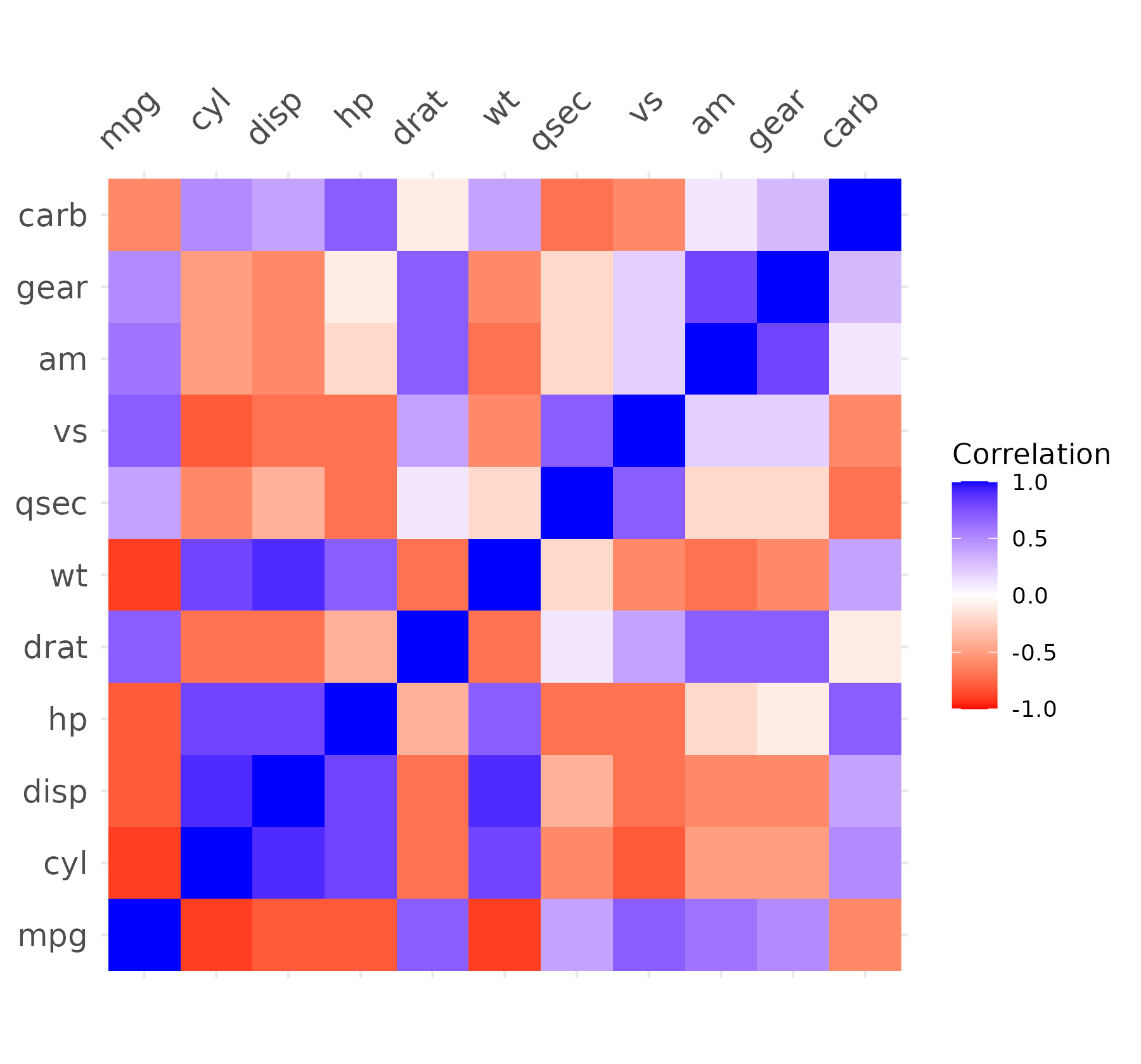

A rectangular predictor-by-outcome matrix

Correlations are not always a square symmetric matrix. To relate one set of variables to another — say engine/size variables against performance variables — pass a rectangular correlation matrix. Clustering and the triangle options need a square matrix, so use hc.order = FALSE.

rect <- round(cor(
  mtcars[, c("mpg", "hp", "wt", "qsec")],
  mtcars[, c("disp", "drat", "vs", "am", "gear")]
), 1)
ggcorrplot(rect, hc.order = FALSE, lab = TRUE, outline.color = "white")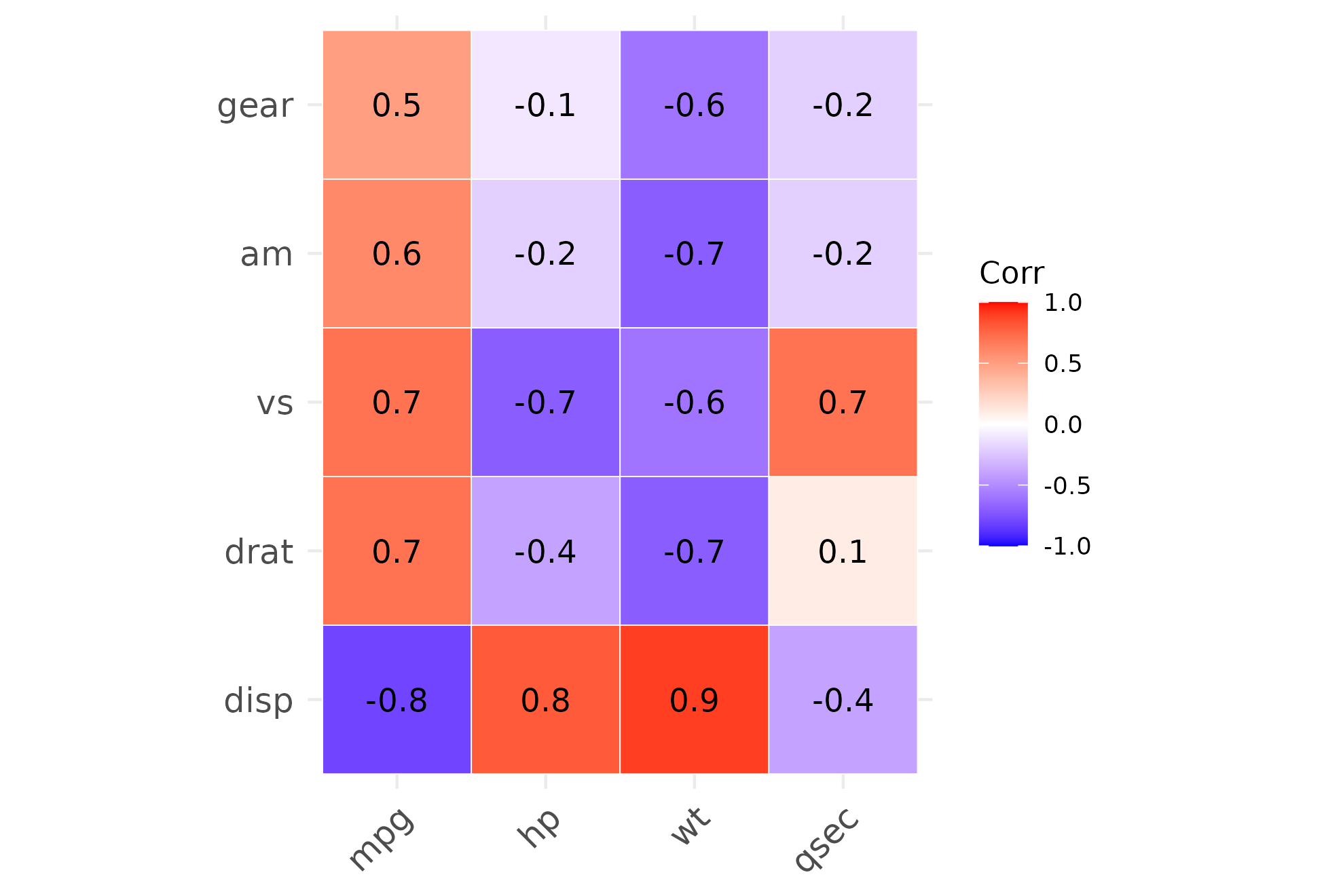

Going further: it is a ggplot

Because ggcorrplot() returns a ggplot object, anything ggplot2 can do is available. Start from any correlogram and add a title, a clearer legend label, and theme tweaks; then save at print resolution.

The legend label is a ggcorrplot argument (legend.title); the title, subtitle and theme come from ggplot2.

p <- ggcorrplot(corr,
  hc.order = TRUE, type = "lower", outline.color = "white",
  legend.title = "Pearson r"
) +
  labs(
    title = "Correlations among car-design variables",
    subtitle = "mtcars, Pearson correlation"
  ) +
  theme(plot.title = element_text(face = "bold"))
p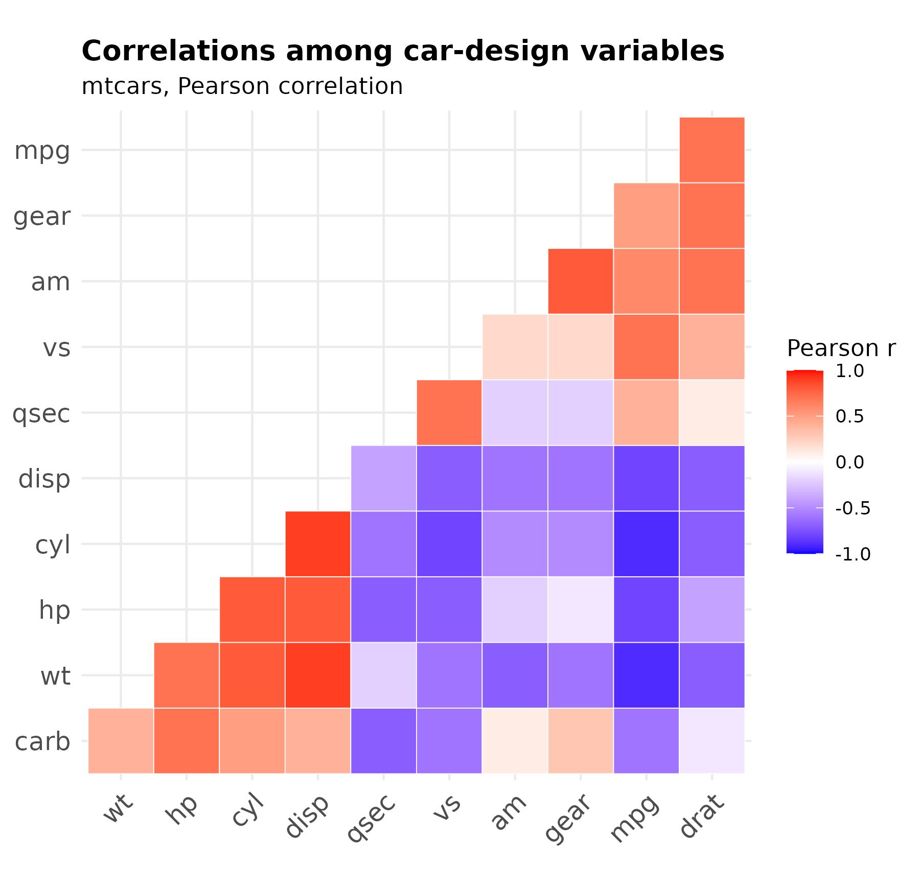

ggsave("correlogram.png", p, width = 7, height = 6, dpi = 300)

Session information

sessionInfo()
#> R version 4.6.1 (2026-06-24)
#> Platform: x86_64-pc-linux-gnu
#> Running under: Ubuntu 24.04.4 LTS
#> 
#> Matrix products: default
#> BLAS:   /usr/lib/x86_64-linux-gnu/openblas-pthread/libblas.so.3 
#> LAPACK: /usr/lib/x86_64-linux-gnu/openblas-pthread/libopenblasp-r0.3.26.so;  LAPACK version 3.12.0
#> 
#> locale:
#>  [1] LC_CTYPE=C.UTF-8       LC_NUMERIC=C           LC_TIME=C.UTF-8       
#>  [4] LC_COLLATE=C.UTF-8     LC_MONETARY=C.UTF-8    LC_MESSAGES=C.UTF-8   
#>  [7] LC_PAPER=C.UTF-8       LC_NAME=C              LC_ADDRESS=C          
#> [10] LC_TELEPHONE=C         LC_MEASUREMENT=C.UTF-8 LC_IDENTIFICATION=C   
#> 
#> time zone: UTC
#> tzcode source: system (glibc)
#> 
#> attached base packages:
#> [1] stats     graphics  grDevices utils     datasets  methods   base     
#> 
#> other attached packages:
#> [1] ggcorrplot_0.3.0 ggplot2_4.0.3   
#> 
#> loaded via a namespace (and not attached):
#>  [1] gtable_0.3.6       jsonlite_2.0.0     dplyr_1.2.1        compiler_4.6.1    
#>  [5] Rcpp_1.1.2         tidyselect_1.2.1   stringr_1.6.0      dichromat_2.0-1   
#>  [9] jquerylib_0.1.4    systemfonts_1.3.2  scales_1.4.0       textshaping_1.0.5 
#> [13] yaml_2.3.12        fastmap_1.2.0      plyr_1.8.9         R6_2.6.1          
#> [17] labeling_0.4.3     generics_0.1.4     knitr_1.51         htmlwidgets_1.6.4 
#> [21] tibble_3.3.1       desc_1.4.3         bslib_0.11.0       pillar_1.11.1     
#> [25] RColorBrewer_1.1-3 rlang_1.3.0        stringi_1.8.7      cachem_1.1.0      
#> [29] xfun_0.60          fs_2.1.0           sass_0.4.10        S7_0.2.2          
#> [33] otel_0.2.0         cli_3.6.6          pkgdown_2.2.1      withr_3.0.3       
#> [37] magrittr_2.0.5     digest_0.6.39      grid_4.6.1         lifecycle_1.0.5   
#> [41] vctrs_0.7.3        evaluate_1.0.5     glue_1.8.1         farver_2.1.2      
#> [45] ragg_1.5.2         reshape2_1.4.5     rmarkdown_2.31     tools_4.6.1       
#> [49] pkgconfig_2.0.3    htmltools_0.5.9

Alboukadel Kassambara