Interpolation function
interp.RdThis function implements bivariate interpolation for irregularly spaced input data. Piecewise linear (=barycentric interpolation), bilinear or bicubic spline interpolation according to Akimas method is applied.
Usage
interp(x, y = NULL, z, xo = seq(min(x), max(x), length = nx),
       yo = seq(min(y), max(y), length = ny),
       linear = (method == "linear"), extrap = FALSE,
       duplicate = "error", dupfun = NULL,
       nx = 40, ny = 40, input="points", output = "grid",
       method = "linear", deltri = "shull", h=0,
       kernel="gaussian", solver="QR", degree=3,
       baryweight=TRUE, autodegree=FALSE, adtol=0.1,
       smoothpde=FALSE, akimaweight=TRUE, nweight=25,
       na.rm=FALSE)
Arguments
- x
vector of \(x\)-coordinates of data points or a
SpatialPointsDataFrameobject (a regular griddedSpatialPixelsDataFrameis also allowed). In this case also an sp data object will be returned. Missing values are not accepted.- y
vector of \(y\)-coordinates of data points. Missing values are not accepted.
If left as NULL indicates that
xshould be aSpatialPointsDataFrameandznames the variable of interest in this dataframe.- z
vector of \(z\)-values at data points or a character variable naming the variable of interest in the
SpatialPointsDataFramex.Missing values are not accepted by default, see parameter
na.rm.x,y, andzmust be the same length (execpt ifxis aSpatialPointsDataFrame) and may contain no fewer than four points. The points ofxandyshould not be collinear ifinput="grid", as the underlying triangulation in these cases sometimes fails.interpis meant for cases in which you have \(x\), \(y\) values scattered over a plane and a \(z\) value for each. If, instead, you are trying to evaluate a mathematical function, or get a graphical interpretation of relationships that can be described by a polynomial, tryouter.- xo
If
output="grid"(which is the default): sequence of \(x\) locations for rectangular output grid, defaults tonxpoints betweenmin(x)andmax(x).If
output="points": vector of \(x\) locations for output points.- yo
If
output="grid"(default): sequence of \(y\) locations for rectangular output grid, defaults tonypoints betweenmin(y)andmax(y).If
output="points": vector of \(y\) locations for output points. In this case it has to be same length asxo.- input
text, possible values are
"grid"(not yet implemented) and"points"(default).This is used to distinguish between regular and irregular gridded input data.
- output
text, possible values are
"grid"(=default) and"points".If
"grid"is choosen thenxoandyoare interpreted as vectors spanning a rectangular grid of points \((xo[i],yo[j])\), \(i=1,...,nx\), \(j=1,...,ny\). This default behaviour matches howakima::interpworks.In the case of
"points"xoandyohave to be of same length and are taken as possibly irregular spaced output points \((xo[i],yo[i])\), \(i=1,...,no\) withno=length(xo).nxandnyare ignored in this case. This case is meant as replacement for the pointwise interpolation done byakima::interpp. If the inputxis aSpatialPointsDataFrameandoutput="points"thenxohas to be aSpatialPointsDataFrame,yowill be ignored.- linear
logical, only for backward compatibility with
akima::interp, indicates if piecewise linear interpolation or Akima splines should be used.Please use the new
methodargument instead!- method
text, possible methods are
"linear"(piecewise linear interpolation within the triangles of the Delaunay triangulation, also referred to as barycentric interpolation based on barycentric coordinates) and"akima"(a reimplementation for Akimas spline algorithms for irregular gridded data with the accuracy of a bicubic polynomial).method="bilinear"is only applicable to regular grids (input="grid") and in turn callsbilinear, see there for more details.method="linear"replaces the oldlinearargument ofakima::interp.- extrap
logical, indicates if extrapolation outside the convex hull is intended, this will not work for piecewise linear interpolation!
- duplicate
character string indicating how to handle duplicate data points. Possible values are
"error"produces an error message,
"strip"remove duplicate z values,
"mean","median","user"calculate mean , median or user defined function (
dupfun) of duplicate \(z\) values.
- dupfun
a function, applied to duplicate points if
duplicate= "user".- nx
dimension of output grid in x direction
- ny
dimension of output grid in y direction
- deltri
triangulation method used, this argument may later be moved into a control set together with others related to the spline interpolation! Possible values are
"shull"(default, sweep hull algorithm) and"deldir"(uses packagedeldir).- h
bandwidth for partial derivatives estimation, compare
locpolyfor details- kernel
kernel for partial derivatives estimation, compare
locpolyfor details- solver
solver used in partial derivatives estimation, compare
locpolyfor details- degree
degree of local polynomial used for partial derivatives estimation, compare
locpolyfor details- baryweight
calculate three partial derivatives estimators and return a barycentric weighted average.
This increases the accuracy of Akima splines but the runtime is multplied by 3!
- autodegree
try to reduce
degreeautomatically- adtol
tolerance used for autodegree
- smoothpde
Use an averaged version of partial derivatives estimates, by default simple average of
nweightestimates.Currently disabled by default (FALSE), underlying code still a bit experimental.
- akimaweight
apply Akima weighting scheme on partial derivatives estimations instead of simply averaging
- nweight
size of search neighbourhood for weighting scheme, default: 25
- na.rm
remove points where z=
NA, defaults toFALSE
Value
a list with 3 components:
- x,y
If
output="grid": vectors of \(x\)- and \(y\)-coordinates of output grid, the same as the input argumentxo, oryo, if present. Otherwise, their default, a vector 40 points evenly spaced over the range of the inputxandy.If
output="points": vectors of \(x\)- and \(y\)-coordinates of output points as given byxoandyo.- z
If
output="grid": matrix of fitted \(z\)-values. The valuez[i,j]is computed at the point \((xo[i], yo[j])\).zhas dimensionslength(xo)timeslength(yo).If
output="points": a vector with the calculated z values for the output points as given byxoandyo.If the input was a
SpatialPointsDataFrameaSpatialPixelsDataFrameis returned foroutput="grid"and aSpatialPointsDataFrameforoutput="points".
References
Moebius, A. F. (1827) Der barymetrische Calcul. Verlag v. Johann Ambrosius Barth, Leipzig, https://books.google.at/books?id=eFPluv_UqFEC&hl=de&pg=PR1#v=onepage&q&f=false
Franke, R., (1979). A critical comparison of some methods for interpolation of scattered data. Tech. Rep. NPS-53-79-003, Dept. of Mathematics, Naval Postgraduate School, Monterey, Calif.
Akima, H. (1978). A Method of Bivariate Interpolation and Smooth Surface Fitting for Irregularly Distributed Data Points. ACM Transactions on Mathematical Software 4, 148-164.
Akima, H. (1996). Algorithm 761: scattered-data surface fitting that has the accuracy of a cubic polynomial. ACM Transactions on Mathematical Software 22, 362–371.
Author
Albrecht Gebhardt <[email protected]>, Roger Bivand <[email protected]>
Note
Please note that this function tries to be a replacement for the interp() function from the akima package. So it should be call compatible for most applications. It also offers additional tuning parameters, usually the default settings will fit. Please be aware that these additional parameters may change in the future as they are still under development.
Examples
### Use all datasets from Franke, 1979:
data(franke)
## x-y irregular grid points:
oldseed <- set.seed(42)
ni <- 64
xi <- runif(ni,0,1)
yi <- runif(ni,0,1)
xyi <- cbind(xi,yi)
## linear interpolation
fi <- franke.fn(xi,yi,1)
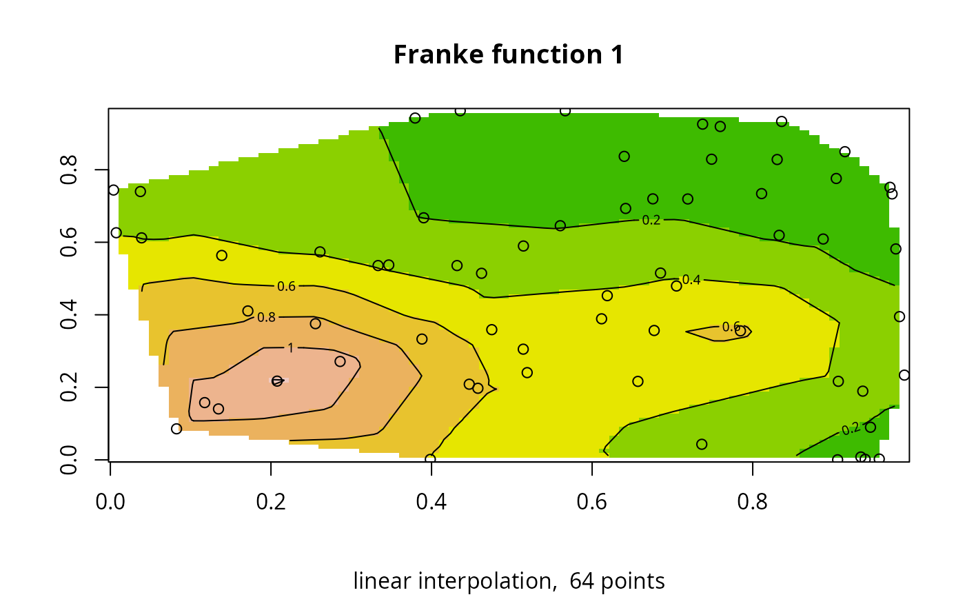
IL <- interp(xi,yi,fi,nx=80,ny=80,method="linear")
## prepare breaks and colors that match for image and contour:
breaks <- pretty(seq(min(IL$z,na.rm=TRUE),max(IL$z,na.rm=TRUE),length=11))
db <- breaks[2]-breaks[1]
nb <- length(breaks)
breaks <- c(breaks[1]-db,breaks,breaks[nb]+db)
colors <- terrain.colors(length(breaks)-1)
image(IL,breaks=breaks,col=colors,main="Franke function 1",
sub=paste("linear interpolation, ", ni,"points"))
contour(IL,add=TRUE,levels=breaks)
points(xi,yi)
 ## spline interpolation
fi <- franke.fn(xi,yi,1)
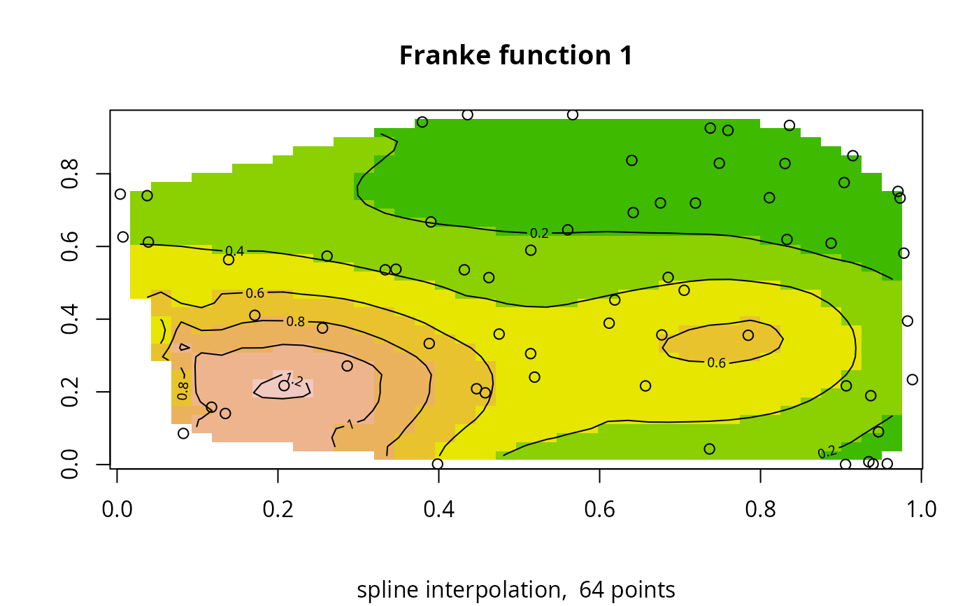
IS <- interp(xi,yi,fi,method="akima",
kernel="gaussian",solver="QR")
## prepare breaks and colors that match for image and contour:
breaks <- pretty(seq(min(IS$z,na.rm=TRUE),max(IS$z,na.rm=TRUE),length=11))
db <- breaks[2]-breaks[1]
nb <- length(breaks)
breaks <- c(breaks[1]-db,breaks,breaks[nb]+db)
colors <- terrain.colors(length(breaks)-1)
image(IS,breaks=breaks,col=colors,main="Franke function 1",
sub=paste("spline interpolation, ", ni,"points"))
contour(IS,add=TRUE,levels=breaks)
points(xi,yi)
## spline interpolation
fi <- franke.fn(xi,yi,1)
IS <- interp(xi,yi,fi,method="akima",
kernel="gaussian",solver="QR")
## prepare breaks and colors that match for image and contour:
breaks <- pretty(seq(min(IS$z,na.rm=TRUE),max(IS$z,na.rm=TRUE),length=11))
db <- breaks[2]-breaks[1]
nb <- length(breaks)
breaks <- c(breaks[1]-db,breaks,breaks[nb]+db)
colors <- terrain.colors(length(breaks)-1)
image(IS,breaks=breaks,col=colors,main="Franke function 1",
sub=paste("spline interpolation, ", ni,"points"))
contour(IS,add=TRUE,levels=breaks)
points(xi,yi)
 ## regular grid:
nx <- 8; ny <- 8
xg<-seq(0,1,length=nx)
yg<-seq(0,1,length=ny)
xx <- t(matrix(rep(xg,ny),nx,ny))
yy <- matrix(rep(yg,nx),ny,nx)
xyg<-expand.grid(xg,yg)
## linear interpolation
fg <- outer(xg,yg,function(x,y)franke.fn(x,y,1))
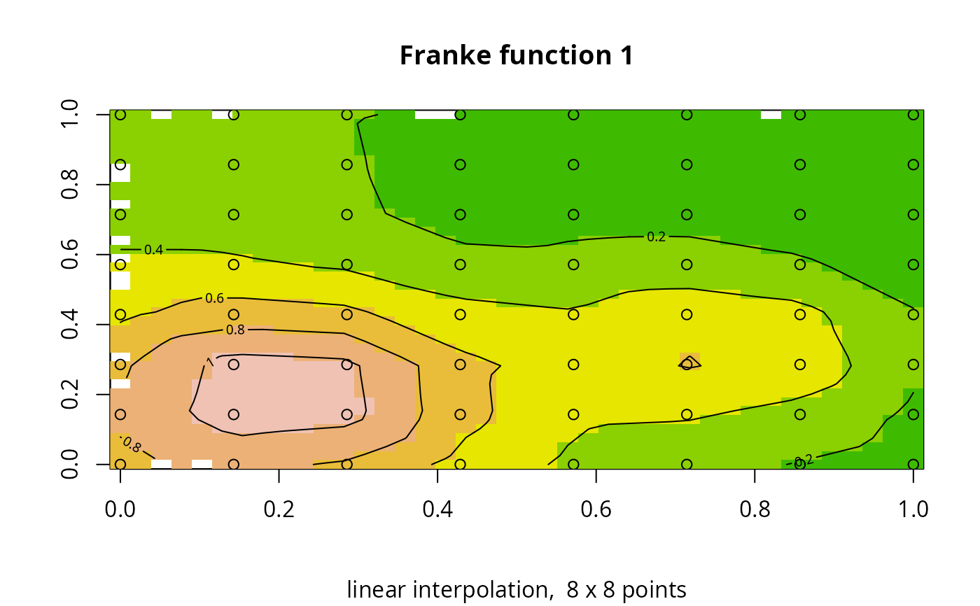
IL <- interp(xg,yg,fg,input="grid",method="linear")
## prepare breaks and colors that match for image and contour:
breaks <- pretty(seq(min(IL$z,na.rm=TRUE),max(IL$z,na.rm=TRUE),length=11))
db <- breaks[2]-breaks[1]
nb <- length(breaks)
breaks <- c(breaks[1]-db,breaks,breaks[nb]+db)
colors <- terrain.colors(length(breaks)-1)
image(IL,breaks=breaks,col=colors,main="Franke function 1",
sub=paste("linear interpolation, ", nx,"x",ny,"points"))
contour(IL,add=TRUE,levels=breaks)
points(xx,yy)
## regular grid:
nx <- 8; ny <- 8
xg<-seq(0,1,length=nx)
yg<-seq(0,1,length=ny)
xx <- t(matrix(rep(xg,ny),nx,ny))
yy <- matrix(rep(yg,nx),ny,nx)
xyg<-expand.grid(xg,yg)
## linear interpolation
fg <- outer(xg,yg,function(x,y)franke.fn(x,y,1))
IL <- interp(xg,yg,fg,input="grid",method="linear")
## prepare breaks and colors that match for image and contour:
breaks <- pretty(seq(min(IL$z,na.rm=TRUE),max(IL$z,na.rm=TRUE),length=11))
db <- breaks[2]-breaks[1]
nb <- length(breaks)
breaks <- c(breaks[1]-db,breaks,breaks[nb]+db)
colors <- terrain.colors(length(breaks)-1)
image(IL,breaks=breaks,col=colors,main="Franke function 1",
sub=paste("linear interpolation, ", nx,"x",ny,"points"))
contour(IL,add=TRUE,levels=breaks)
points(xx,yy)
 ## spline interpolation
fg <- outer(xg,yg,function(x,y)franke.fn(x,y,1))
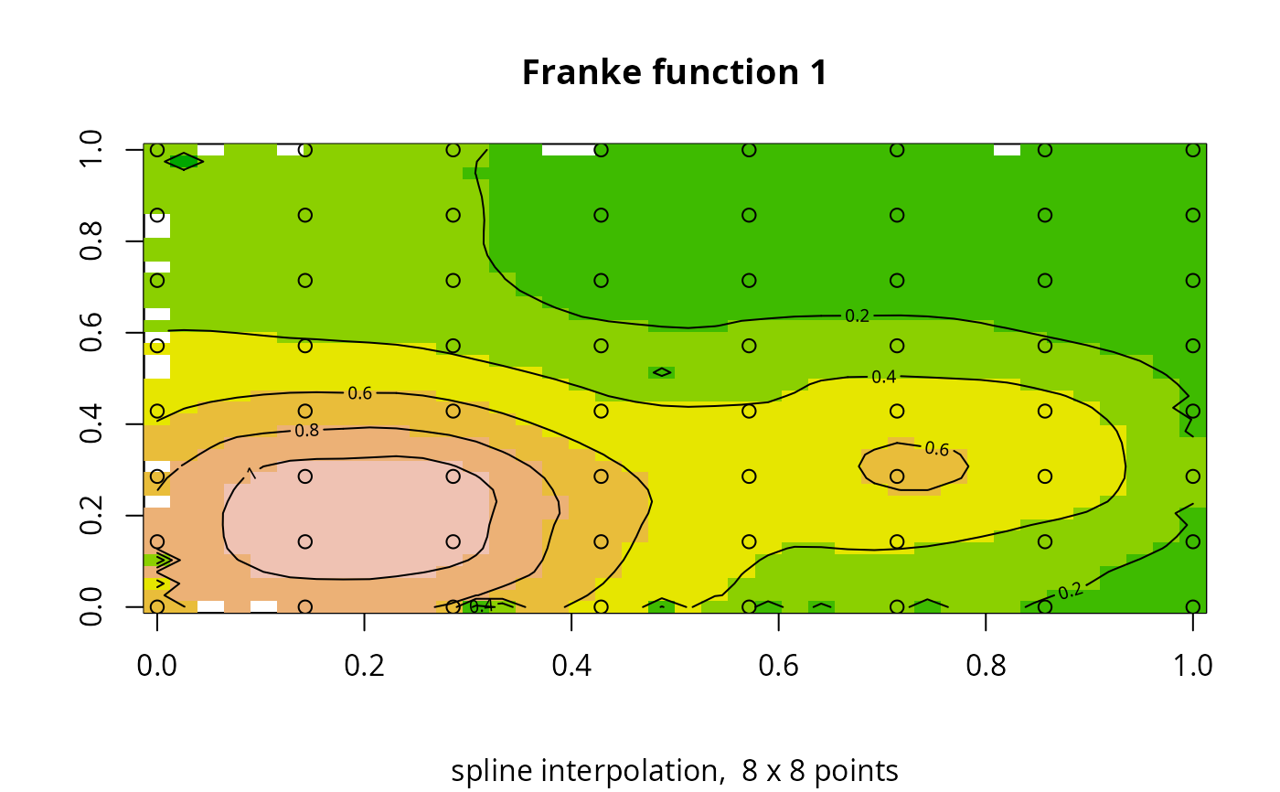
IS <- interp(xg,yg,fg,input="grid",method="akima",
kernel="gaussian",solver="QR")
## prepare breaks and colors that match for image and contour:
breaks <- pretty(seq(min(IS$z,na.rm=TRUE),max(IS$z,na.rm=TRUE),length=11))
db <- breaks[2]-breaks[1]
nb <- length(breaks)
breaks <- c(breaks[1]-db,breaks,breaks[nb]+db)
colors <- terrain.colors(length(breaks)-1)
image(IS,breaks=breaks,col=colors,main="Franke function 1",
sub=paste("spline interpolation, ", nx,"x",ny,"points"))
contour(IS,add=TRUE,levels=breaks)
points(xx,yy)
## spline interpolation
fg <- outer(xg,yg,function(x,y)franke.fn(x,y,1))
IS <- interp(xg,yg,fg,input="grid",method="akima",
kernel="gaussian",solver="QR")
## prepare breaks and colors that match for image and contour:
breaks <- pretty(seq(min(IS$z,na.rm=TRUE),max(IS$z,na.rm=TRUE),length=11))
db <- breaks[2]-breaks[1]
nb <- length(breaks)
breaks <- c(breaks[1]-db,breaks,breaks[nb]+db)
colors <- terrain.colors(length(breaks)-1)
image(IS,breaks=breaks,col=colors,main="Franke function 1",
sub=paste("spline interpolation, ", nx,"x",ny,"points"))
contour(IS,add=TRUE,levels=breaks)
points(xx,yy)
 ## apply interp to sp data:
require(sp)
#> Loading required package: sp
## convert Akima data set to a sp object
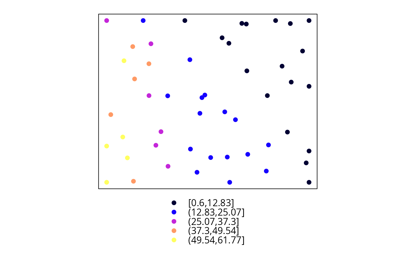
data(akima)
asp <- SpatialPointsDataFrame(list(x=akima$x,y=akima$y),
data = data.frame(z=akima$z))
spplot(asp,"z")
## apply interp to sp data:
require(sp)
#> Loading required package: sp
## convert Akima data set to a sp object
data(akima)
asp <- SpatialPointsDataFrame(list(x=akima$x,y=akima$y),
data = data.frame(z=akima$z))
spplot(asp,"z")
 ## linear interpolation
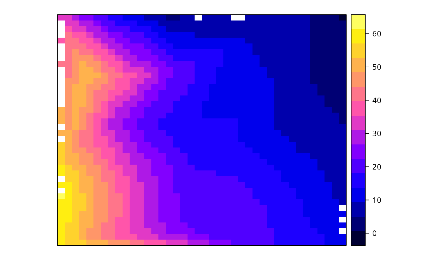
spli <- interp(asp, z="z", method="linear")
## the result is again a SpatialPointsDataFrame:
spplot(spli,"z")
## linear interpolation
spli <- interp(asp, z="z", method="linear")
## the result is again a SpatialPointsDataFrame:
spplot(spli,"z")
 ## now with spline interpolation, slightly higher resolution
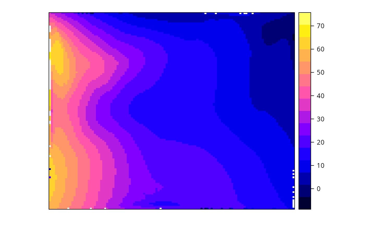
spsi <- interp(asp, z="z", method="akima", nx=120, ny=120)
spplot(spsi,"z")
## now with spline interpolation, slightly higher resolution
spsi <- interp(asp, z="z", method="akima", nx=120, ny=120)
spplot(spsi,"z")
 ## now sp grids: reuse stuff from above
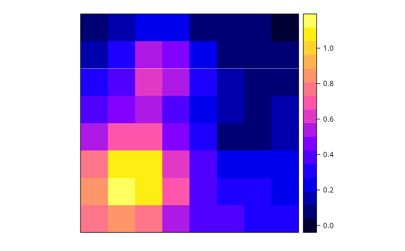
spgr <- SpatialPixelsDataFrame(list(x=c(xx),y=c(yy)),
data=data.frame(z=c(fg)))
spplot(spgr)
## now sp grids: reuse stuff from above
spgr <- SpatialPixelsDataFrame(list(x=c(xx),y=c(yy)),
data=data.frame(z=c(fg)))
spplot(spgr)
 ## linear interpolation
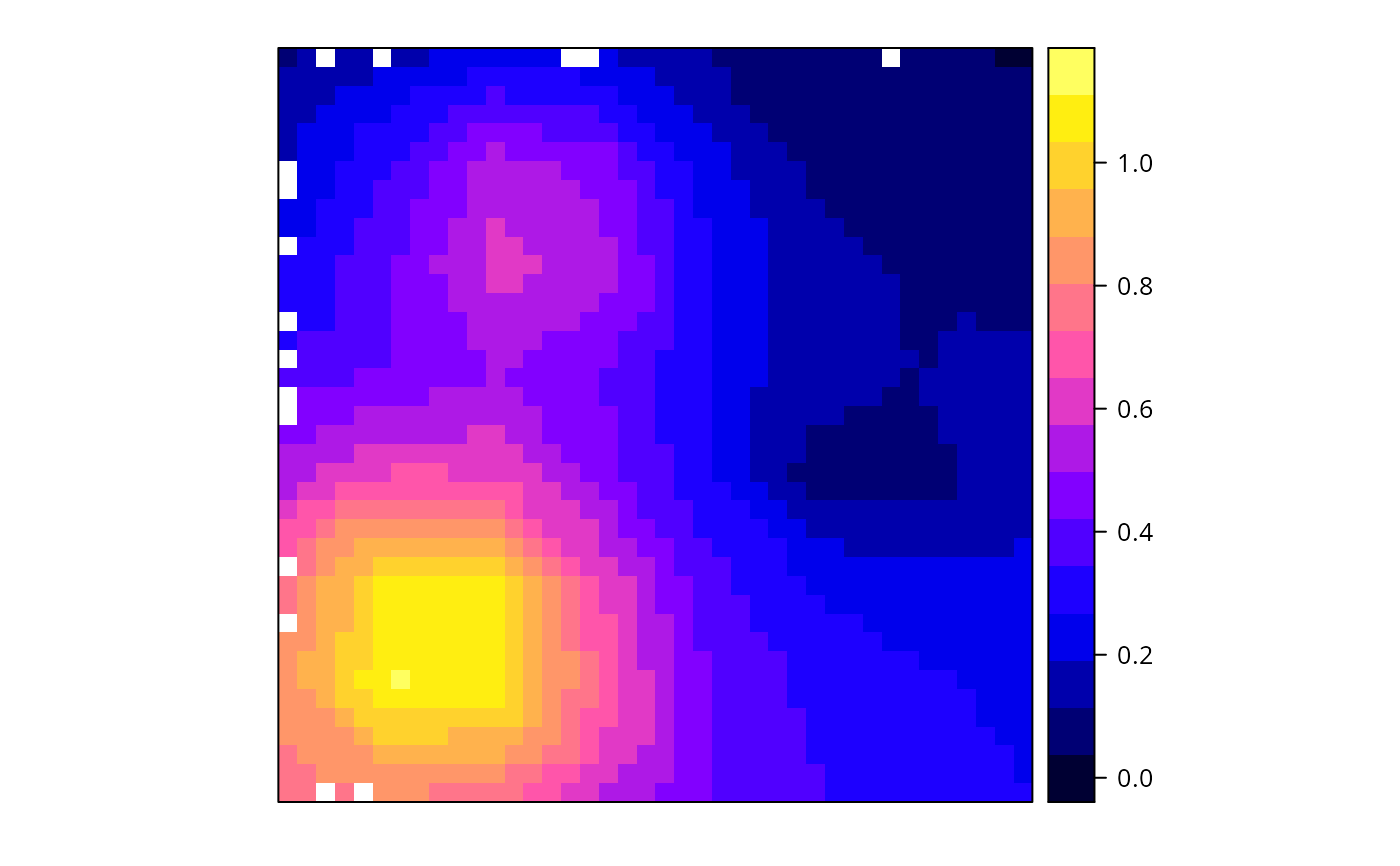
spli <- interp(spgr, z="z", method="linear", input="grid")
## the result is again a SpatialPointsDataFrame:
spplot(spli,"z")
## linear interpolation
spli <- interp(spgr, z="z", method="linear", input="grid")
## the result is again a SpatialPointsDataFrame:
spplot(spli,"z")
 ## now with spline interpolation, slightly higher resolution
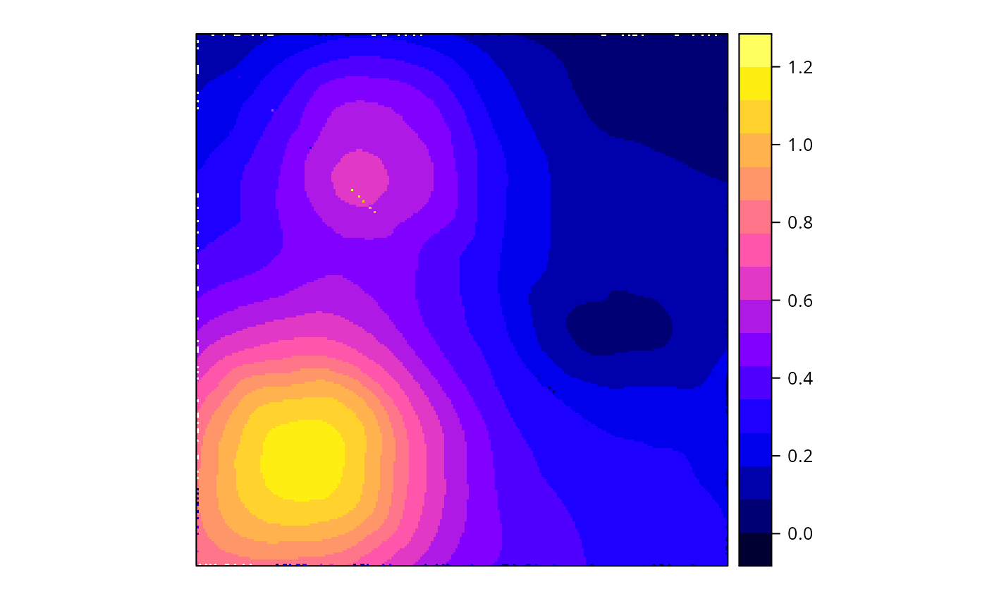
spsi <- interp(spgr, z="z", method="akima", nx=240, ny=240)
spplot(spsi,"z")
## now with spline interpolation, slightly higher resolution
spsi <- interp(spgr, z="z", method="akima", nx=240, ny=240)
spplot(spsi,"z")
 set.seed(oldseed)