Introduction
The current version of lme4 offers four covariance
classes/structures: Covariance.us (unstructured),
Covariance.diag (diagonal), Covariance.cs
(compound symmetry), and Covariance.ar1 (autoregressive
order 1). The syntax for use is somewhat similar to the
glmmTMB package (see covariance
structures in glmmTMB), although the results are slightly
different.
The first half of this vignette provide a more detailed explanation
of how the new machinery works, and the second half of the vignette will
compare lme4 and glmmTMB implementations and
results.
Background
For exact details of this structure, refer to the lmer
vignette
(Bates et al. 2015). We provide a quick
summary in this vignette.
In matrix notation, a linear mixed model can be represented as: Where represents an unknown vector of random effects. The class helps define the structure of the variance-covariance matrix as specified as . Typically, we denote the variance-covariance matrix as .
First, we create the relative co-factor
which is a
block diagonal matrix that depends on the variance-component parameter
.
Let
be the scale parameter of the variance of a linear mixed model. In
lme4, the variance-covariance matrix is constructed by:
For generalized linear mixed models, instead represents the unscaled Cholesky factor; that is, the scaling term is omitted from the equation above.
The major difference between the four covariance classes
(Covariance.us (unstructured), Covariance.diag
(diagonal), Covariance.cs (compound symmetry), and
Covariance.ar1 (autoregressive order 1)) is the
construction of the the relative Cholesky factor
.
Covariance Structures
Suppose there are
number of random effect terms for a particular grouping variable. The
unstructured covariance, which is the default in
lme4, of size
has the following form:
The next three covariance structures can either be heterogeneous or
homogeneous. If we have a homogeneous covariance structure
(hom = TRUE), then we assume
.
The diagonal covariance has the following form: By default, we assume a heterogeneous diagonal covariance structure.
The compound symmetric covariance has the following form: By default, we assume a heterogeneous compound symmetric covariance structure.
The AR1 (auto-regressive order 1) covariance has the following form: Unlike the diagonal and compound symmetric structures, by default we assume a homogeneous ar1 covariance structure.
Construction of the Relative Co-factor
For the unstructured covariance matrix, lme4 estimates
the following parameters in par:
to construct the relative co-factor
(this is the same as in previous versions):
The definition of the parameter vectors differs for the other
covariance structures. In the diagonal covariance matrix case,
(or par) only contains the standard deviations. The
relative co-factor
is:
For the compound symmetry covariance structure, the parameter vector
par contains the
standard deviations
and the common correlation
.
In contrast to glmmTMB, the correlation is estimated on its
original scale (bounded between -1 and 1), rather than on an
unconstrained, transformed scale.
The relative co-factor is a lower triangular matrix. Consider the form:
Its elements are constructed as follows. First, define the sequence recursively:
Then the elements of
are given by:
In the code, one can extract the values
via the getTheta() function of the
Covariance.cs object, in which theta will be a
vector in the column-wise elements of
.
The setup is similar for the autoregressive order 1 (AR1) covariance structure. Again, the parameter vector contains the standard deviations and the autocorrelation parameter . The relative co-factor is a lower triangular matrix whose form is similar to the compound symmetric case.
The elements
are given by:
Again, these values can be extracted
using getTheta() function of the
Covariance.ar1 object, in which theta will be
still be a vector in the column-wise elements of
.
Extracting model components
This section illustrates how to extract par,
theta, Lambda, as described in the previous
section, as well as the variance covariance matrices of a model, from a
merMod object.
We’ll fit the standard sleepstudy example, except that
we will use a model with a compound symmetric covariance structure.
Because this model has only two varying effects (intercept and slope
with respect to day) per subject, and hence the covariance matrix is
,
there is no difference in overall model fit between the
compound-symmetric and the unstructured covariance matrices. Howevever,
the models are parameterized differently, so this example will highlight
the differences between par and theta.
library(lme4)
#> Loading required package: Matrix
fm1.cs <- lmer(Reaction ~ Days + cs(1 + Days | Subject), sleepstudy)
Extracting the covariance structure:
print(fm1.cs_cov <- getReCovs(fm1.cs))
#> [[1]]
#> An object of class "Covariance.cs"
#> Slot "hom":
#> [1] FALSE
#>
#> Slot "nc":
#> [1] 2
#>
#> Slot "par":
#> [1] 0.96679232 0.23140420 0.06561148
The result is a list with only one element as we only have one
random-effects term (cs(1 + Days | Subject)). To see the
values of par and theta for this object, we
can call:
getME(fm1.cs, "par")
#> Subject.(Intercept)        Subject.Days         Subject.rho
#>          0.96679232          0.23140420          0.06561148
getME(fm1.cs, "theta")
#>      Subject.(Intercept) Subject.Days.(Intercept)             Subject.Days
#>               0.96679232               0.01518277               0.23090558
The matrix is large, so we’ll view it instead of printing:
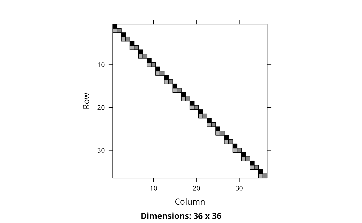
To most users, the most crucial information is simply the
variance-covariance matrices. Extracte these via
VarCorr.merMod() (the list has one element per
random-effect term in the model — in this case, only one):
vc_mat <- VarCorr(fm1.cs)
vc_mat$Subject
#>             (Intercept)      Days
#> (Intercept)  612.160273  9.613533
#> Days           9.613533 35.070443
#> attr(,"class")
#> [1] "vcmat_cs" "matrix"   "array"
#> attr(,"stddev")
#> [1] 24.74187  5.92203
#> attr(,"correlation")
#>             (Intercept)       Days
#> (Intercept)  1.00000000 0.06561148
#> Days         0.06561148 1.00000000
#> attr(,"theta")
#> [1] 0.96679232 0.01518277 0.23090558
#> attr(,"profpar")
#> [1] 0.96679232 0.23140420 0.06561148
#> attr(,"rho")
#> [1] 0.06561148
Comparisons with glmmTMB
Reason for Computational Differences
When fitting linear mixed models, lme4 parameterizes the
random-effects variance–covariance matrix on an unconstrained scale,
using box-constrained optimization algorithms to ensure that the
variance-covariance matrix is positive semidefinite. For unstructured
covariance matrices, this means that the elements of
that parameterize the diagonal elements of
are constrained to be
(for diagonal models, all of the elements of
fill the diagonal of
and hence are
;
for models such as the compound-symmetric or AR1 models that use
correlation parameters, we constrain
.
As discussed in Bates et al. (2015), this
constrained parameterization works well for handling model where the
estimated covariance matrix is singular
(i.e.
is only positive semidefinite, not positive definite). In addition, for
linear mixed models lme4 profiles the fixed-effect
parameters out of the objective function (Bates
et al. 2015); finally, the scale parameter
is not estimated directly, but is derived from the residual variance or
deviance of the fitted model.
In contrast, glmmTMB uses direct maximum likelihood
estimation via Template Model Builder (TMB), fitting to the full
parameter vector
.
Covariance parameters are fitted on a transformed (unconstrained) scale:
log scale for standard deviations and various scales for correlation
parameters (see the glmmTMB covariance
structures vignette for details). This parameterization simplifies
fitting (a box-constrained algorithm isn’t necessary), but is less
convenient in singular fits and other cases where the maximum likelihood
estimate is infinite on the unconstrained scale.
Despite these differences, we will show examples where
lme4 and glmmTMB provide similar estimates
when they both use maximum likelihood estimation. By default,
lme4 uses the restricted maximum likelihood; hence in the
following examples, we use lmer(..., REML = FALSE) to
compare against glmmTMB.
Comparison Setup
if (!requireNamespace("glmmTMB", quietly = TRUE)) {
  knitr::opts_chunk$set(eval = FALSE)
} else {
  library(glmmTMB)
}

## Often want to ignore attributes and class.
## Set a fairly large tolerance for convenience.
all.equal.nocheck <- function(x, y, tolerance = 3e-5, ..., check.attributes = FALSE, check.class = FALSE) {
  require("Matrix", quietly = TRUE)
  ## working around mode-matching headaches
  if (is(x, "Matrix")) x <- matrix(x)
  if (is(y, "Matrix")) y <- matrix(y)
  all.equal(x, y, ..., tolerance = tolerance, check.attributes = check.attributes, check.class = check.class)
}

get.cor1 <- function(x) {
  v <- VarCorr(x)
  vv <- if (inherits(x, "merMod")) v$group else v$cond$group
  attr(vv, "correlation")[1,2]
}
Unstructured (General Positive Definite)
This is the default setting for both lme4 and
glmmTMB. Below we simulate a dataset with known
beta, theta and sigma values.
n_groups <- 20
n_per_group <- 20
n <- n_groups * n_per_group

set.seed(1)
dat.us <- data.frame(
  group = rep(1:n_groups, each = n_per_group),
  x1 = rnorm(n),
  x2 = rnorm(n)
)
## Constructing a similar dataset for the other examples
gdat.us <- dat.diag <- gdat.diag <- dat.us

form <- y ~ 1 + x1 * x2 + us(1 + x1|group)
dat.us$y <- simulate(form[-2],
                    newdata = dat.us,
                    family = gaussian,
                    newparams = list(beta = c(-7, 5, -100, 20),
                                     theta = c(2.5, 1.4, 6.3),
                                     sigma = 2))[[1]]

form2 <- y ~ 1 + x1 + us(1 + x1|group)
gdat.us$y <- simulate(
  form2[-2],
  newdata = gdat.us,
  family = binomial,
  newparams = list(
    beta  = c(-1.5, 0.5),
    theta = c(0.3, 0.1, 0.3)
  ))[[1]]
Linear Mixed Model
lme4.us <- lmer(form, data = dat.us, REML = "FALSE")
glmmTMB.us <- glmmTMB(form, dat = dat.us)

## Fixed effects
fixef(lme4.us); fixef(glmmTMB.us)$cond
#> (Intercept)          x1          x2       x1:x2
#>   -7.280739    5.795443 -100.070859   19.958369
#> (Intercept)          x1          x2       x1:x2
#>   -7.280736    5.795388 -100.070860   19.958369
all.equal.nocheck(fixef(lme4.us), fixef(glmmTMB.us)$cond)
#> [1] TRUE

## Sigma
sigma(lme4.us); sigma(glmmTMB.us)
#> [1] 2.049702
#> [1] 2.049702
all.equal.nocheck(sigma(lme4.us), sigma(glmmTMB.us))
#> [1] TRUE

## Log likelihoods
logLik(lme4.us); logLik(glmmTMB.us)
#> 'log Lik.' -971.3046 (df=8)
#> 'log Lik.' -971.3046 (df=8)
all.equal.nocheck(logLik(lme4.us), logLik(glmmTMB.us))
#> [1] TRUE
As expected, calculations related to the random-effects term differ slightly beyond this point.
## Variance-Covariance Matrix
vcov(lme4.us); vcov(glmmTMB.us)$cond
#> 4 x 4 Matrix of class "dpoMatrix"
#>               (Intercept)            x1            x2         x1:x2
#> (Intercept)  1.2015013379 -0.1733524625  0.0008614781 -0.0004201163
#> x1          -0.1733524625 12.4136628944 -0.0008710084  0.0026046011
#> x2           0.0008614781 -0.0008710084  0.0101254478 -0.0018079150
#> x1:x2       -0.0004201163  0.0026046011 -0.0018079150  0.0117364494
#>               (Intercept)            x1            x2         x1:x2
#> (Intercept)  1.2014959308 -0.1733102259  0.0008614825 -0.0004201922
#> x1          -0.1733102259 12.4138803799 -0.0008713988  0.0026042335
#> x2           0.0008614825 -0.0008713988  0.0101257004 -0.0018074214
#> x1:x2       -0.0004201922  0.0026042335 -0.0018074214  0.0117377999
all.equal.nocheck(vcov(lme4.us), vcov(glmmTMB.us)$cond)
#> [1] TRUE

## Variance and Covariance Components
all.equal.nocheck(VarCorr(lme4.us)$group,
          VarCorr(glmmTMB.us)$cond$group)
#> [1] TRUE

## Conditional Modes of the Random Effects
all.equal.nocheck(ranef(lme4.us)$group, ranef(glmmTMB.us)$cond$group)
#> [1] TRUE
Generalized Linear Mixed Model
glme4.us <- glmer(form2, data = gdat.us, family = binomial)
gglmmTMB.us <- glmmTMB(form2, dat = gdat.us, family = binomial)

## Fixed effects
fixef(glme4.us); fixef(gglmmTMB.us)$cond
#> (Intercept)          x1
#>  -1.5400786   0.4547925
#> (Intercept)          x1
#>  -1.5403288   0.4545996
all.equal.nocheck(fixef(glme4.us), fixef(gglmmTMB.us)$cond)
#> [1] "Mean relative difference: 0.0002221048"

## Sigma
all.equal.nocheck(sigma(glme4.us), sigma(gglmmTMB.us))
#> [1] TRUE

## Log likelihoods
logLik(glme4.us); logLik(gglmmTMB.us)
#> 'log Lik.' -191.8811 (df=5)
#> 'log Lik.' -191.8809 (df=5)
all.equal.nocheck(logLik(glme4.us), logLik(gglmmTMB.us))
#> [1] TRUE
As expected, calculations related to the random-effects term differ slightly beyond this point.
## Variance-Covariance Matrix
vcov(glme4.us); vcov(gglmmTMB.us)$cond
#> 2 x 2 Matrix of class "dpoMatrix"
#>              (Intercept)           x1
#> (Intercept)  0.028221233 -0.001848413
#> x1          -0.001848413  0.038084198
#>              (Intercept)           x1
#> (Intercept)  0.028453808 -0.001749237
#> x1          -0.001749237  0.038270693
all.equal.nocheck(vcov(glme4.us), vcov(gglmmTMB.us)$cond)
#> [1] "Mean relative difference: 0.008820021"

## Variance and Covariance Components
all.equal.nocheck(VarCorr(glme4.us)$group,
          VarCorr(gglmmTMB.us)$cond$group)
#> [1] "Mean relative difference: 0.001268453"

## Conditional Modes of the Random Effects
all.equal.nocheck(ranef(glme4.us)$group, ranef(gglmmTMB.us)$cond$group)
#> [1] "Component \"(Intercept)\": Mean relative difference: 0.0009258143"
#> [2] "Component \"x1\": Mean relative difference: 0.0007570482"
Diagonal
The syntax is the same for fitting a heterogeneous diagonal
covariance structure for lme4 and glmmTMB. It
changes when we want to fit a homogeneous diagonal covariance
structure.
To fit a homogeneous diagonal covariance structure we would write:
lme4.us <- lmer(Reaction ~ Days + diag(Days | Subject, hom = TRUE), sleepstudy)
glmmTMB.us <- glmmTMB(Reaction ~ Days + homdiag(Days | Subject), sleepstudy)
We will focus on comparisons of an estimated heterogeneous diagonal covariance structure.
form <- y ~ 1 + x1 * x2 + diag(1|group)
dat.diag$y <- simulate(form[-2],
                       newdata = dat.diag,
                       family = gaussian,
                       newparams = list(beta = c(-7, 5, -100, 20),
                                        theta = c(2.5),
                                        sigma = 2))[[1]]
lme4.diag <- lmer(form, data = dat.diag, REML = "FALSE")
glmmTMB.diag <- glmmTMB(form, dat = dat.diag)

## Fixed effects
fixef(lme4.diag); fixef(glmmTMB.diag)$cond
#> (Intercept)          x1          x2       x1:x2
#>   -6.484337    5.111952 -100.045319   20.037624
#> (Intercept)          x1          x2       x1:x2
#>   -6.484329    5.111952 -100.045319   20.037624
all.equal.nocheck(fixef(lme4.diag), fixef(glmmTMB.diag)$cond)
#> [1] TRUE

## Sigma
sigma(lme4.diag); sigma(glmmTMB.diag)
#> [1] 2.156913
#> [1] 2.156913
all.equal.nocheck(sigma(lme4.diag), sigma(glmmTMB.diag))
#> [1] TRUE

## Log likelihoods
logLik(lme4.diag); logLik(glmmTMB.diag)
#> 'log Lik.' -915.8749 (df=6)
#> 'log Lik.' -915.8749 (df=6)
all.equal.nocheck(logLik(lme4.diag), logLik(glmmTMB.diag))
#> [1] TRUE

## Variance-Covariance Matrix
vcov(lme4.diag); vcov(glmmTMB.diag)$cond
#> 4 x 4 Matrix of class "dpoMatrix"
#>               (Intercept)            x1            x2         x1:x2
#> (Intercept)  0.6899487466 -0.0006448103  0.0008535087 -0.0005702566
#> x1          -0.0006448103  0.0135575383 -0.0008171565  0.0025591747
#> x2           0.0008535087 -0.0008171565  0.0107715407 -0.0021874630
#> x1:x2       -0.0005702566  0.0025591747 -0.0021874630  0.0115262417
#>               (Intercept)            x1            x2         x1:x2
#> (Intercept)  0.6899487512 -0.0006448095  0.0008535098 -0.0005702545
#> x1          -0.0006448095  0.0135576594 -0.0008169500  0.0025595384
#> x2           0.0008535098 -0.0008169500  0.0107718878 -0.0021868490
#> x1:x2       -0.0005702545  0.0025595384 -0.0021868490  0.0115273226
all.equal.nocheck(vcov(lme4.diag), vcov(glmmTMB.diag)$cond)
#> [1] TRUE

## Variance and Covariance Components
all.equal.nocheck(VarCorr(lme4.diag)[[1]],
          VarCorr(glmmTMB.diag)$cond$group)
#> [1] TRUE

## Conditional Modes of the Random Effects
all.equal.nocheck(ranef(lme4.diag)$group, ranef(glmmTMB.diag)$cond$group)
#> [1] TRUE
Compound Symmetry
Similar to the diagonal case, the syntax is the same for fitting a
heterogeneous compound symmetry covariance structure for
lme4 and glmmTMB:
lme4.us <- lmer(Reaction ~ Days + cs(Days | Subject, hom = TRUE), sleepstudy)
glmmTMB.us <- glmmTMB(Reaction ~ Days + cs(Days | Subject), sleepstudy)
Again, it differs when we want to fit a homogeneous compound symmetry covariance structure, which we will use for our comparisons.
simGroup <- function(g, n=6, phi=0.6) {
  x <- MASS::mvrnorm(mu = rep(0,n),
                     Sigma = phi^as.matrix(dist(1:n)) )
  y <- x + rnorm(n)
  times <- factor(1:n)
  group <- factor(rep(g,n))
  data.frame(y, times, group)
}

set.seed(1)
dat.cs <- do.call("rbind", lapply(1:2000, simGroup))
lme4.cs <- lmer(y ~ times + cs(0 + times | group, hom = TRUE), data = dat.cs, REML = FALSE)
glmmTMB.cs <- glmmTMB(y ~ times + homcs(0 + times | group), data = dat.cs)
#> Warning in finalizeTMB(TMBStruc, obj, fit, h, data.tmb.old): Model convergence
#> problem; non-positive-definite Hessian matrix. See vignette('troubleshooting')

## Fixed effects
fixef(lme4.cs); fixef(glmmTMB.cs)$cond
#>  (Intercept)       times2       times3       times4       times5       times6
#> -0.003601028  0.024047964  0.004877225  0.052026751  0.049632430  0.058705282
#>  (Intercept)       times2       times3       times4       times5       times6
#> -0.003614815  0.024054555  0.004889497  0.052034066  0.049639781  0.058721255
all.equal.nocheck(fixef(lme4.cs), fixef(glmmTMB.cs)$cond)
#> [1] "Mean relative difference: 0.0003281084"

## Sigma
sigma(lme4.cs); sigma(glmmTMB.cs)
#> [1] 1.006676
#> [1] 1.041604
all.equal.nocheck(sigma(lme4.cs), sigma(glmmTMB.cs))
#> [1] "Mean relative difference: 0.03469571"

## Log likelihoods
logLik(lme4.cs); logLik(glmmTMB.cs)
#> 'log Lik.' -20850.22 (df=18)
#> 'log Lik.' NA (df=9)
all.equal.nocheck(logLik(lme4.cs), logLik(glmmTMB.cs))
#> [1] "'is.NA' value mismatch: 1 in current 0 in target"

## Variance-Covariance Matrix
all.equal.nocheck(vcov(lme4.cs), vcov(glmmTMB.cs)$cond)
#> [1] TRUE

## Variance and Covariance Components
all.equal.nocheck(VarCorr(lme4.cs)[[1]],
          VarCorr(glmmTMB.cs)$cond$group)
#> [1] "Mean relative difference: 0.02558092"

## Conditional Modes of the Random Effects
all.equal.nocheck(ranef(lme4.cs)$group, ranef(glmmTMB.cs)$cond$group)
#> Warning in sqrt(as.numeric(object$diag.cov.random)): NaNs produced
#> [1] "Component \"times1\": Mean relative difference: 0.07526032"
#> [2] "Component \"times2\": Mean relative difference: 0.07067102"
#> [3] "Component \"times3\": Mean relative difference: 0.06907266"
#> [4] "Component \"times4\": Mean relative difference: 0.06931966"
#> [5] "Component \"times5\": Mean relative difference: 0.07089414"
#> [6] "Component \"times6\": Mean relative difference: 0.0742481"

## Comparing against the predicted rho value
lme4.rho <- get.cor1(lme4.cs)
glmmTMB.rho <- get.cor1(glmmTMB.cs)
lme4.rho; glmmTMB.rho
#> [1] 0.3642212
#> [1] 0.3925468
all.equal.nocheck(lme4.rho, glmmTMB.rho)
#> [1] "Mean relative difference: 0.07777033"
Autoregressive Order 1
For this comparison, we focus on a simulated data set with .
Unlike the diagonal and compound symmetry case, the syntax differs
for fitting either a heterogeneous or a homogeneous AR1 model for
lme4 and glmmTMB.
For a heterogeneous AR1 covariance structure we would write the following:
lme4.ar1 <- lmer(y ~ times + ar1(0 + times | group), data = dat.ar1, REML = FALSE)
glmmTMB.ar1 <- glmmTMB(y ~ times + hetar1(0 + times | group), data = dat.ar1)
We will instead focus on comparisons for a homogeneous AR1 covariance structure.
lme4.ar1 <- lmer(y ~ times + ar1(0 + times | group, hom = TRUE), data = dat.ar1, REML = FALSE)
glmmTMB.ar1 <- glmmTMB(y ~ times + ar1(0 + times | group), data = dat.ar1)

## Fixed effects
fixef(lme4.ar1); fixef(glmmTMB.ar1)$cond
#> (Intercept)      times2      times3      times4      times5      times6
#> -0.01013620  0.02737776  0.02097931  0.07361698  0.05848662  0.05164259
#> (Intercept)      times2      times3      times4      times5      times6
#> -0.01015168  0.02740053  0.02099352  0.07362919  0.05850250  0.05165057
all.equal.nocheck(fixef(lme4.ar1), fixef(glmmTMB.ar1)$cond)
#> [1] "Mean relative difference: 0.0003654732"

## Sigma
sigma(lme4.ar1); sigma(glmmTMB.ar1)
#> [1] 0.9870569
#> [1] 0.9870552
all.equal.nocheck(sigma(lme4.ar1), sigma(glmmTMB.ar1))
#> [1] TRUE

## Log likelihoods
logLik(lme4.ar1); logLik(glmmTMB.ar1)
#> 'log Lik.' -20483.65 (df=18)
#> 'log Lik.' -20483.65 (df=9)
all.equal.nocheck(logLik(lme4.ar1), logLik(glmmTMB.ar1))
#> [1] TRUE

## Variance-Covariance Matrix
all.equal.nocheck(vcov(lme4.ar1), vcov(glmmTMB.ar1)$cond)
#> [1] TRUE

## Variance and Covariance Components
all.equal.nocheck(VarCorr(lme4.ar1)$group,
                  VarCorr(glmmTMB.ar1)$cond$group)
#> [1] TRUE

## Conditional Modes of the Random Effects
all.equal.nocheck(ranef(lme4.ar1)$group, ranef(glmmTMB.ar1)$cond$group)
#> [1] TRUE

## Comparing against the predicted rho value
lme4.ar1.rho <- get.cor1(lme4.ar1)
glmmTMB.ar1.rho <- get.cor1(glmmTMB.ar1)
lme4.ar1.rho; glmmTMB.ar1.rho
#> [1] 0.6821726
#> [1] 0.6821689
all.equal.nocheck(lme4.ar1.rho, glmmTMB.ar1.rho)
#> [1] TRUE