Plots mathematical expressions in one and two variables.
Usage
plotFun(
  object,
  ...,
  plot = trellis.last.object(),
  add = NULL,
  under = FALSE,
  xlim = NULL,
  ylim = NULL,
  npts = NULL,
  ylab = NULL,
  xlab = NULL,
  zlab = NULL,
  filled = TRUE,
  levels = NULL,
  nlevels = 10,
  labels = TRUE,
  surface = FALSE,
  groups = NULL,
  col = trellis.par.get("superpose.line")$col,
  col.regions = topo.colors,
  type = "l",
  lwd = trellis.par.get("superpose.line")$lwd,
  lty = trellis.par.get("superpose.line")$lty,
  alpha = NULL,
  discontinuities = NULL,
  discontinuity = 1,
  interactive = rstudio_is_available()
)
Arguments
- object
a mathematical expression or a function "of one variable" which will converted to something intuitively equivalent to
object(x) ~ x. (See examples)- ...
additional parameters, typically processed by
latticefunctions such aslattice::xyplot(),lattice::levelplot()or their panel functions. Frequently used parameters includemainmain title for plot
subsubtitle for plot
lwdline width
ltyline type
cola color or a (small) integer indicating which color in the current color scheme is desired.
Additionally, these arguments can be used to specify parameters for the function being plotted and to specify the plotting window with natural names. See the examples for such usage.
- plot
a trellis object; by default, the most recently created trellis plot. When
addisTRUE, the new function will be plotted into a layer added to this object.- add
if
TRUE, then add a layer to an existing plot rather than creating a new plot. IfNULL, this will be determined by the value ofunder.- under
if
TRUE, then new layer is added beneath existing layers- xlim
limits for x axis (or use variable names, see examples)
- ylim
limits for y axis (or use variable names, see examples)
- npts
number of points for plotting.
- ylab
label for y axis
- xlab
label for x axis
- zlab
label for z axis (when in surface-plot mode)
- filled
fill with color between the contours (
TRUEby default)- levels
levels at which to draw contours
- nlevels
number of contours to draw (if
levelsnot specified)- labels
if
FALSE, don't label contours- surface
draw a surface plot rather than a contour plot
- groups
grouping argument ala lattice graphics
- col
vector of colors for line graphs and contours
- col.regions
a vector of colors or a function (
topo.colorsby default) for generating such- type
type of plot (
"l"by default)- lwd
vector of line widths for line graphs
- lty
vector of line types for line graphs
- alpha
number from 0 (transparent) to 1 (opaque) for the fill colors
- discontinuities
a vector of input values at which a function is discontinuous or
NULLto use a heuristic to auto-detect.- discontinuity
a positive number determining how sensitive the plot is to potential discontinuity. Larger values result in less sensitivity. The default is 1. Use
discontinuity = Infto disable discontinuity detection. Discontinuity detection uses a crude numerical heuristic and may not give the desired results in all cases.- interactive
a logical indicating whether the surface plot should be interactive.
Details
makes plots of mathematical expressions using the formula syntax. Will
draw both line plots and contour/surface plots (for functions of two variables).
In RStudio, the surface plot comes with sliders to set orientation.
If the colors in filled surface plots are too blocky, increase npts
beyond the default of 50, though npts=300 is as much as you're likely to ever need.
See examples for overplotting a constraint function on an objective function.
Examples
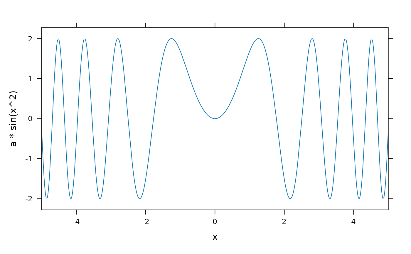
plotFun( a*sin(x^2)~x, xlim=range(-5,5), a=2 ) # setting parameter value
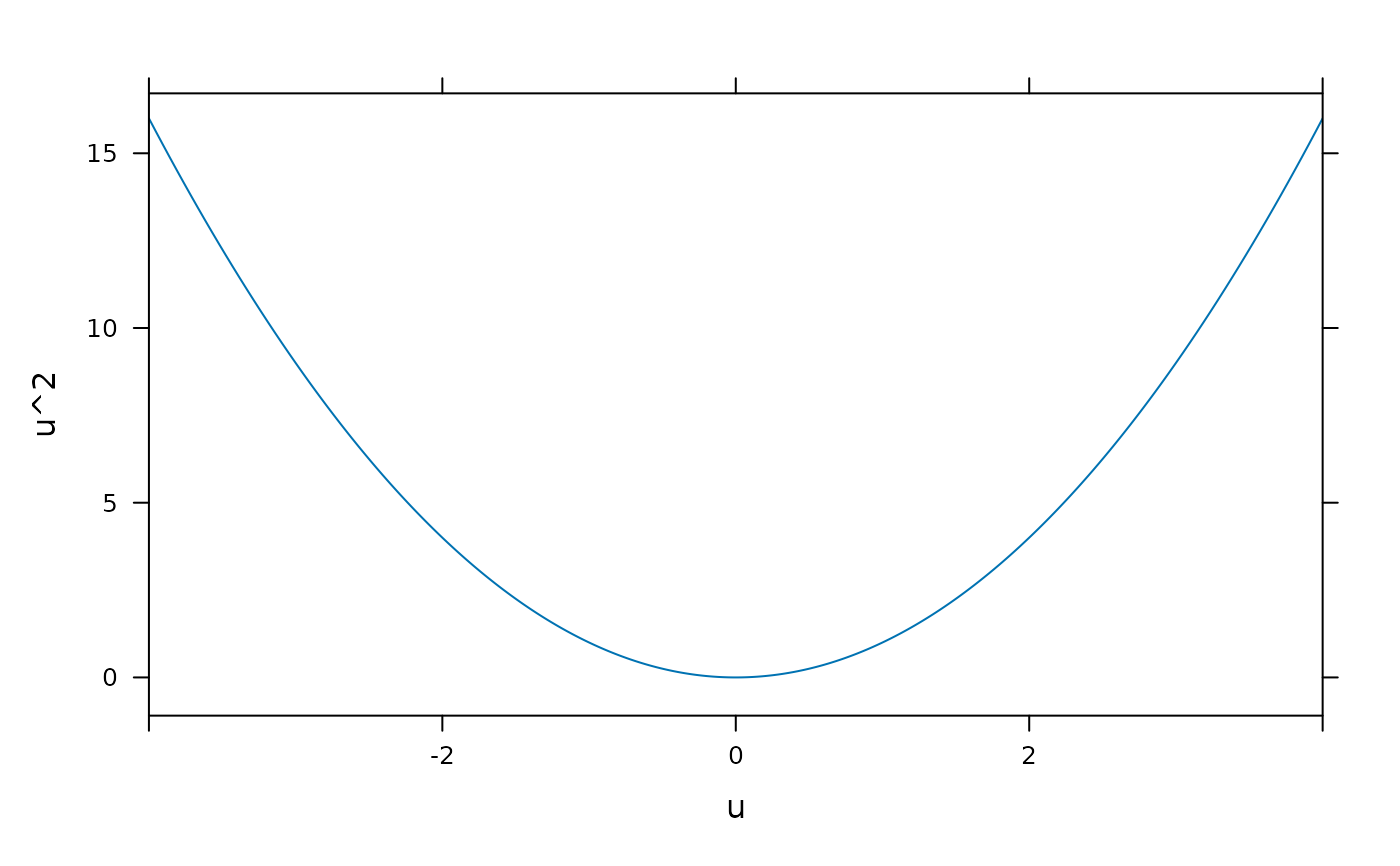
 plotFun( u^2 ~ u, ulim=c(-4,4) ) # limits in terms of u
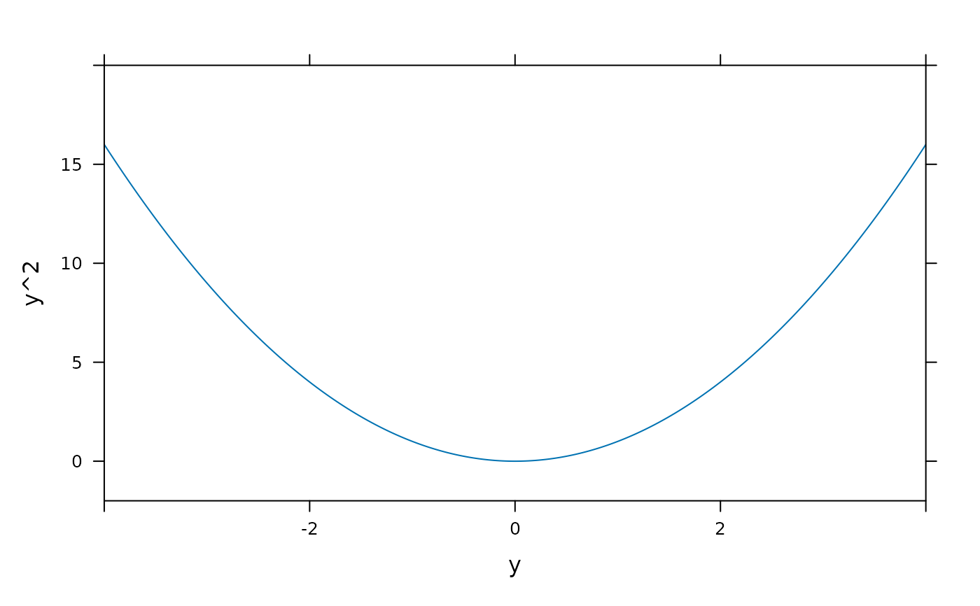
 # Note roles of ylim and y.lim in this example
plotFun( y^2 ~ y, ylim=c(-2,20), y.lim=c(-4,4) )
# Note roles of ylim and y.lim in this example
plotFun( y^2 ~ y, ylim=c(-2,20), y.lim=c(-4,4) )
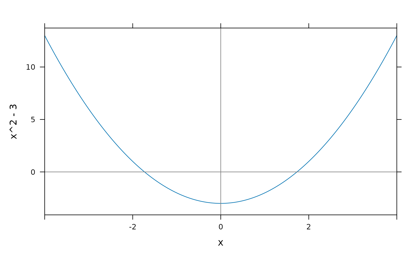
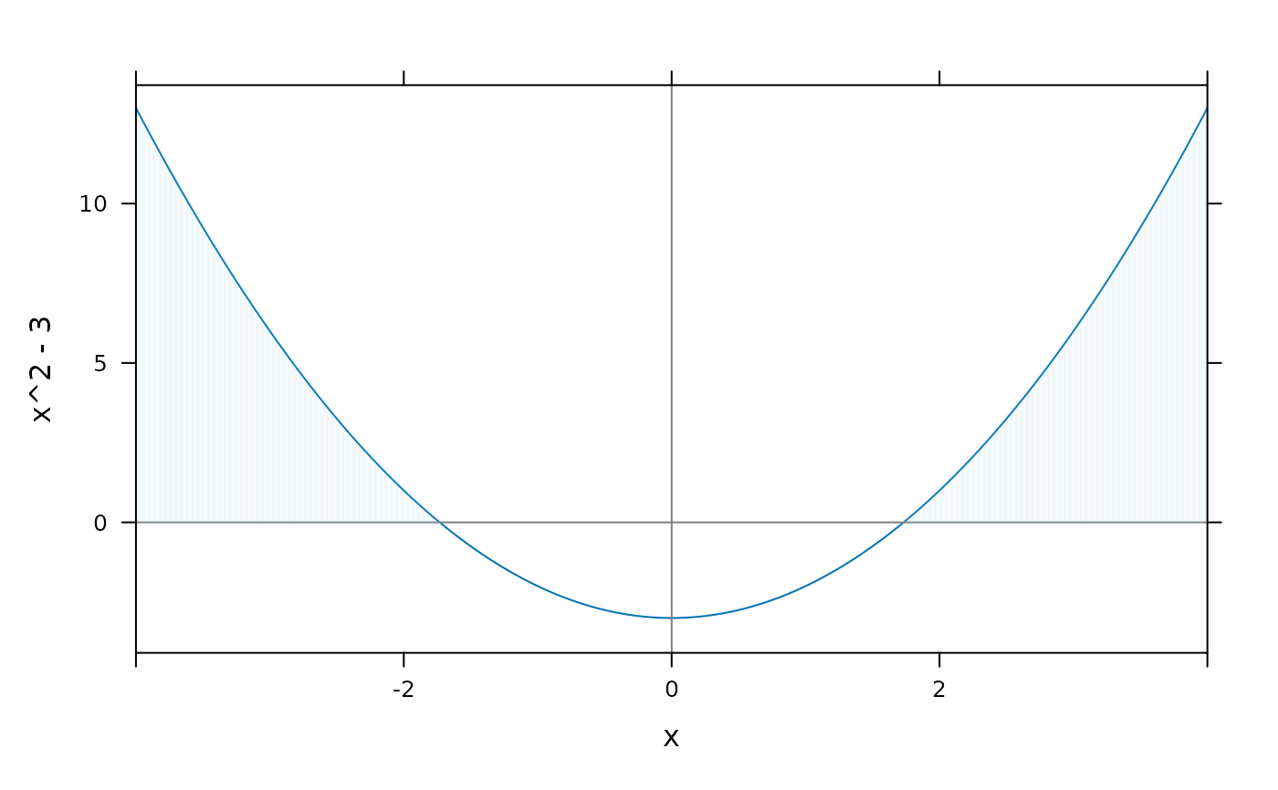
 # Combining plot elements to show the solution to an inequality
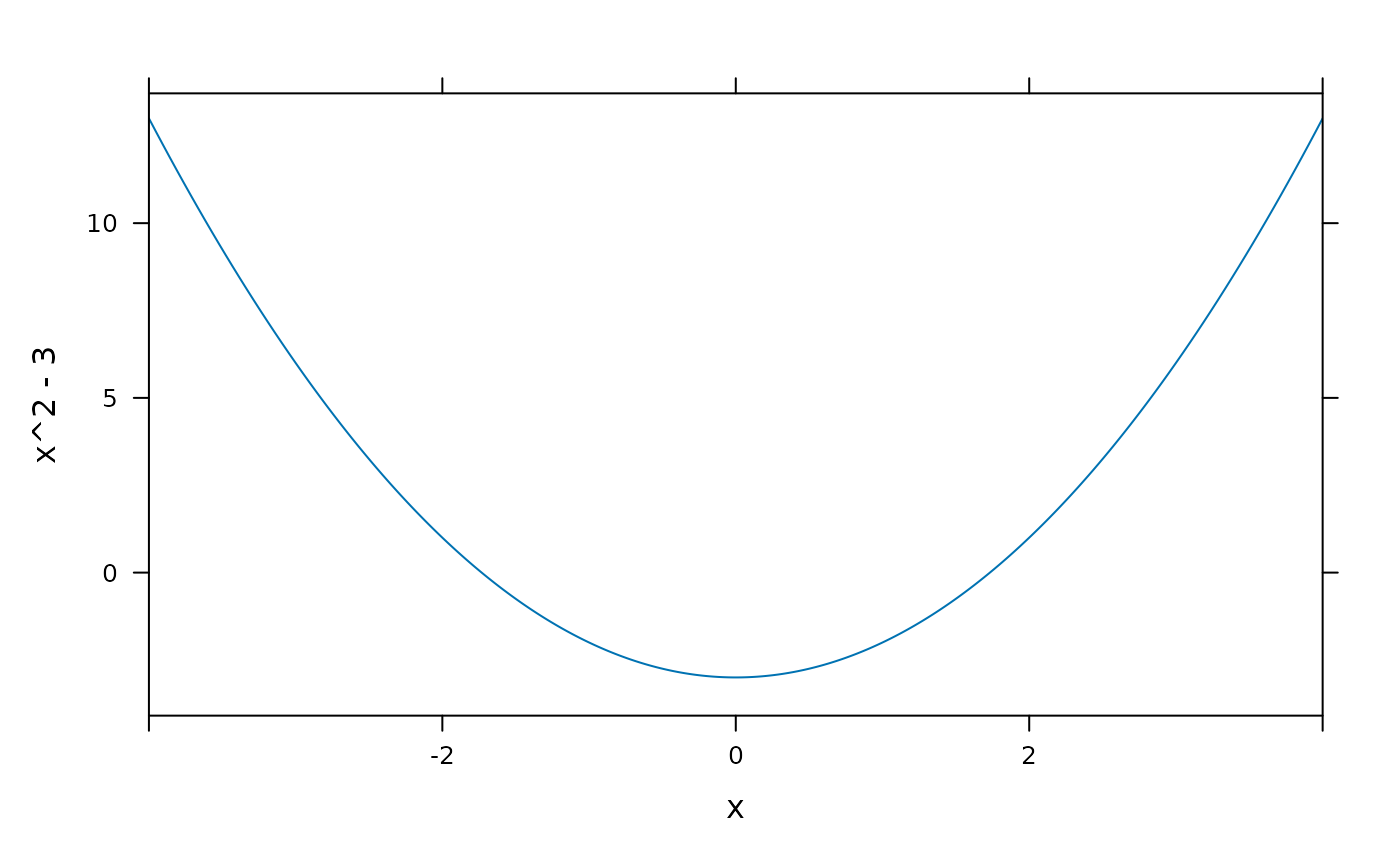
plotFun( x^2 -3 ~ x, xlim=c(-4,4), grid=TRUE )
# Combining plot elements to show the solution to an inequality
plotFun( x^2 -3 ~ x, xlim=c(-4,4), grid=TRUE )
 ladd( panel.abline(h=0,v=0,col='gray50') )
 plotFun( (x^2 -3) * (x^2 > 3) ~ x, type='h', alpha=.1, lwd=4, col='lightblue', add=TRUE )
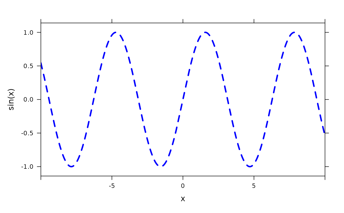
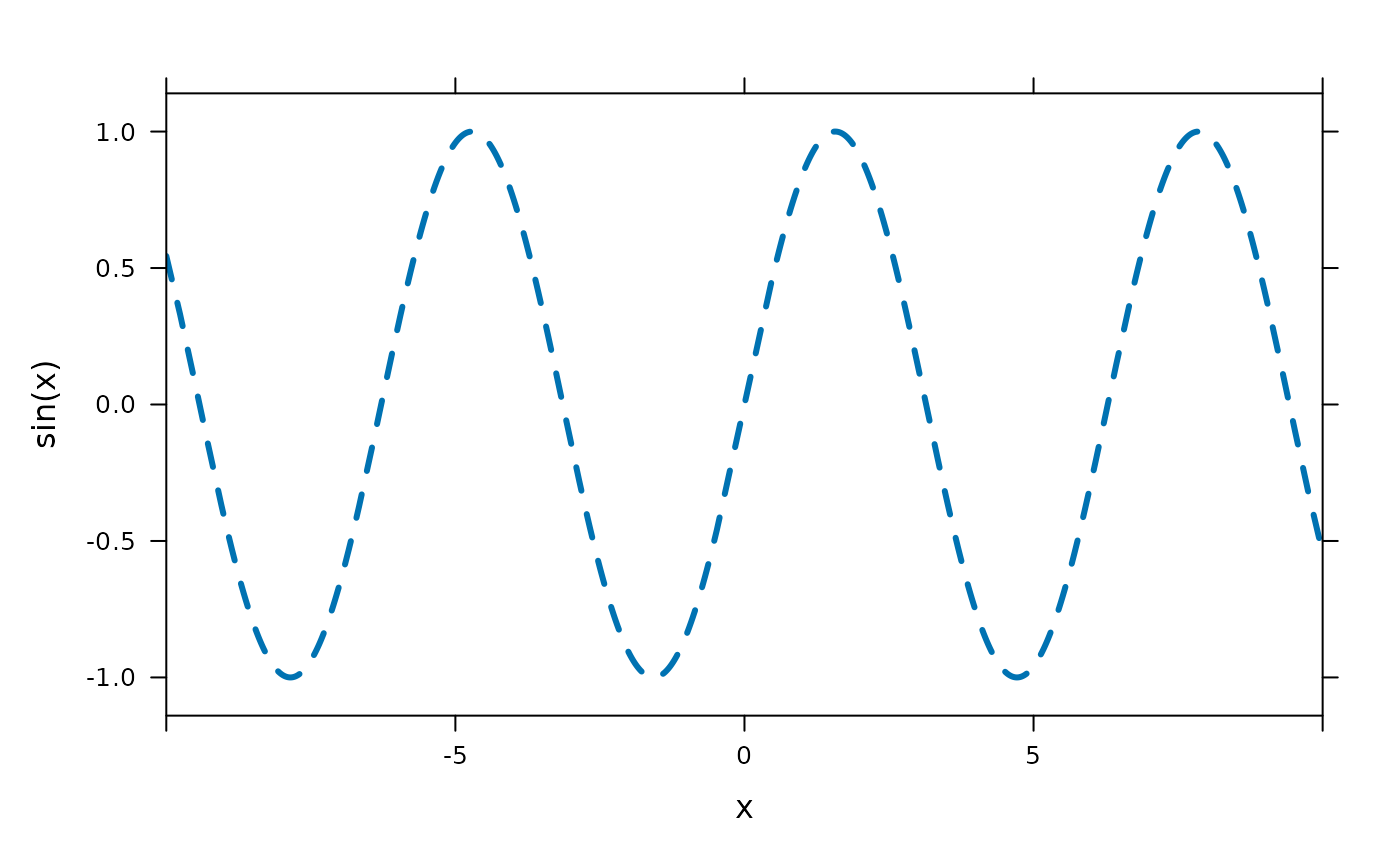
 plotFun( sin(x) ~ x,
groups=cut(x, findZeros(sin(x) ~ x, within=10)$x),
col=c('blue','green'), lty=2, lwd=3, xlim=c(-10,10) )
plotFun( sin(x) ~ x,
groups=cut(x, findZeros(sin(x) ~ x, within=10)$x),
col=c('blue','green'), lty=2, lwd=3, xlim=c(-10,10) )
 plotFun( sin(x) ~ x,
groups=cut(x, findZeros(sin(x) ~ x, within=10)$x),
col=c(1,2), lty=2, lwd=3, xlim=c(-10,10) )
#> converting numerical color value into a color using lattice settings
plotFun( sin(x) ~ x,
groups=cut(x, findZeros(sin(x) ~ x, within=10)$x),
col=c(1,2), lty=2, lwd=3, xlim=c(-10,10) )
#> converting numerical color value into a color using lattice settings
 ## plotFun( sin(2*pi*x/P)*exp(-k*t)~x+t, k=2, P=.3)
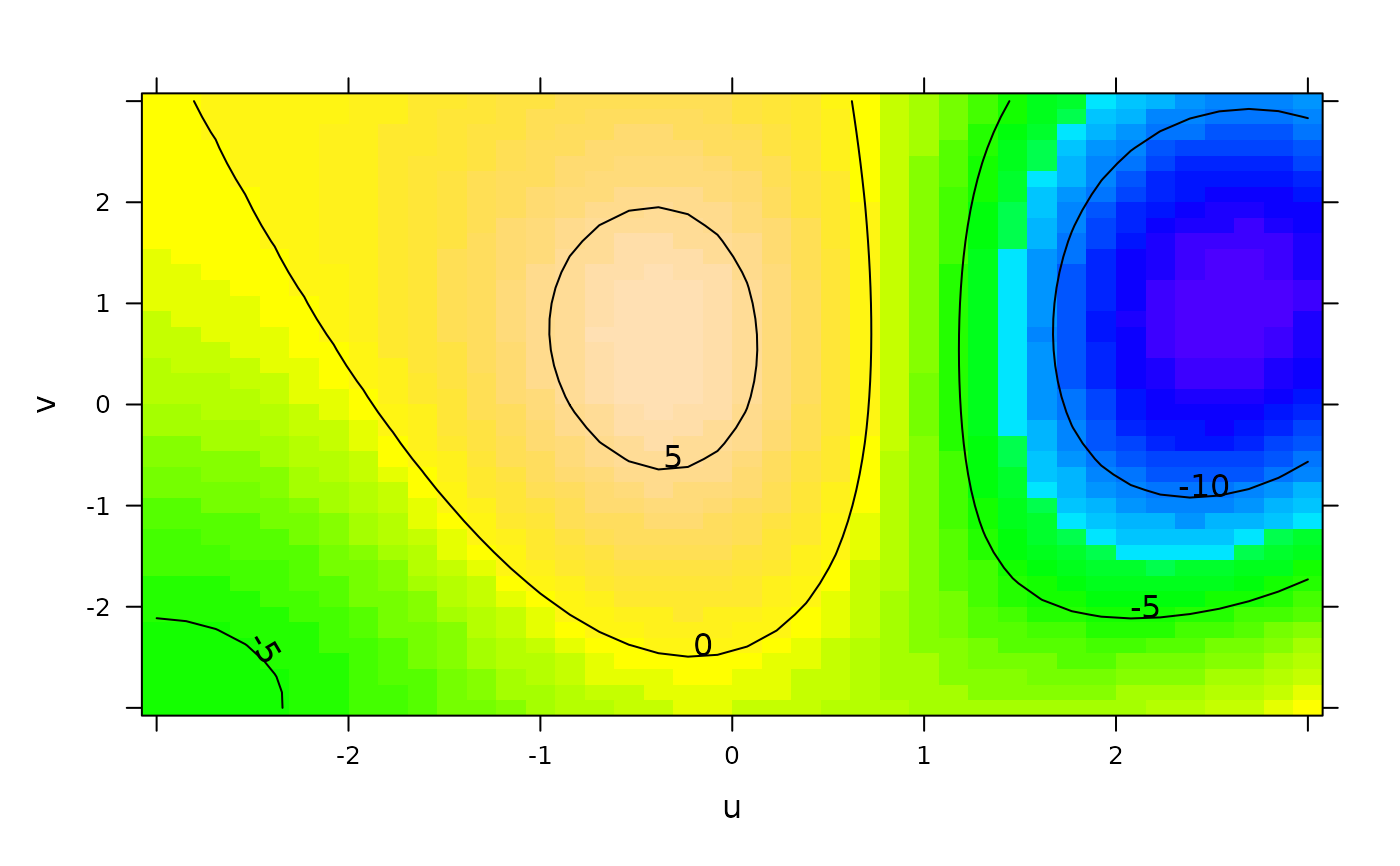
f <- rfun( ~ u & v )
plotFun( f(u=u,v=v) ~ u & v, u.lim=range(-3,3), v.lim=range(-3,3) )
## plotFun( sin(2*pi*x/P)*exp(-k*t)~x+t, k=2, P=.3)
f <- rfun( ~ u & v )
plotFun( f(u=u,v=v) ~ u & v, u.lim=range(-3,3), v.lim=range(-3,3) )
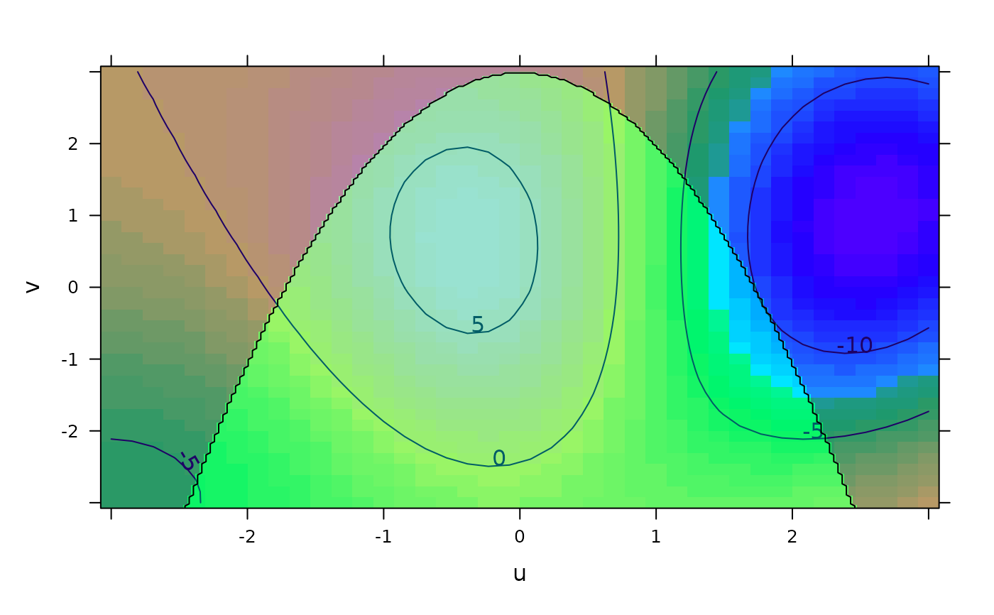
 plotFun( u^2 + v < 3 ~ u & v, add=TRUE, npts=200 )
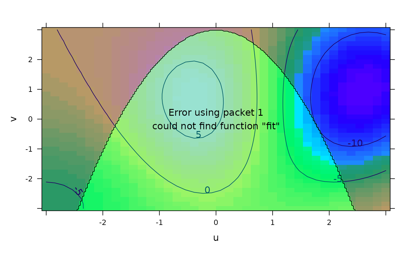
 if (require(mosaicData)) {
# display a linear model using a formula interface
model <- lm(wage ~ poly(exper,degree=2), data=CPS85)
fit <- makeFun(model)
xyplot(wage ~ exper, data=CPS85)
plotFun(fit(exper) ~ exper, add=TRUE, lwd=3, col="red")
# Can also just give fit since it is a "function of one variable"
plotFun(fit, add=TRUE, lwd=2, col='white')
}
if (require(mosaicData)) {
# display a linear model using a formula interface
model <- lm(wage ~ poly(exper,degree=2), data=CPS85)
fit <- makeFun(model)
xyplot(wage ~ exper, data=CPS85)
plotFun(fit(exper) ~ exper, add=TRUE, lwd=3, col="red")
# Can also just give fit since it is a "function of one variable"
plotFun(fit, add=TRUE, lwd=2, col='white')
}
 # Attempts to find sensible axis limits by default
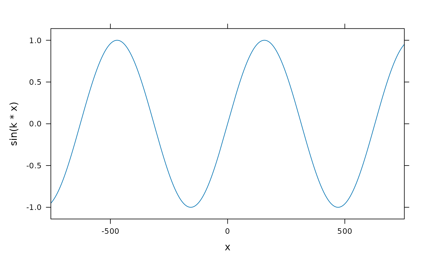
plotFun( sin(k*x)~x, k=0.01 )
# Attempts to find sensible axis limits by default
plotFun( sin(k*x)~x, k=0.01 )
 # Plotting a linear model with multiple predictors.
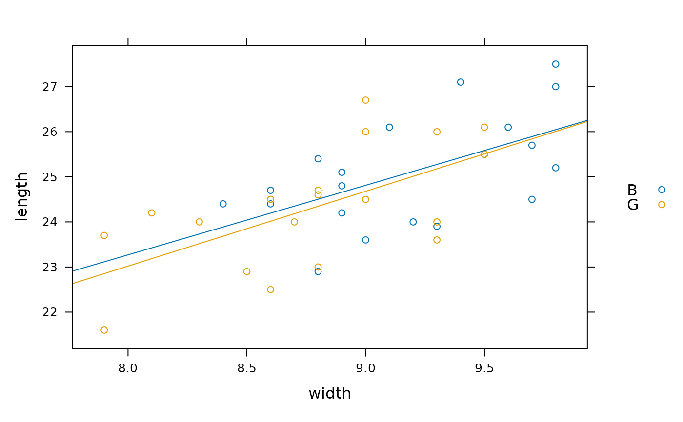
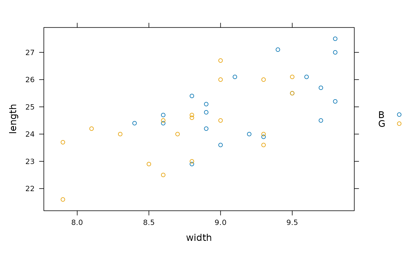
mod <- lm(length ~ width * sex, data=KidsFeet)
fitted.length <- makeFun(mod)
xyplot(length ~ width, groups=sex, data=KidsFeet, auto.key=TRUE)
# Plotting a linear model with multiple predictors.
mod <- lm(length ~ width * sex, data=KidsFeet)
fitted.length <- makeFun(mod)
xyplot(length ~ width, groups=sex, data=KidsFeet, auto.key=TRUE)
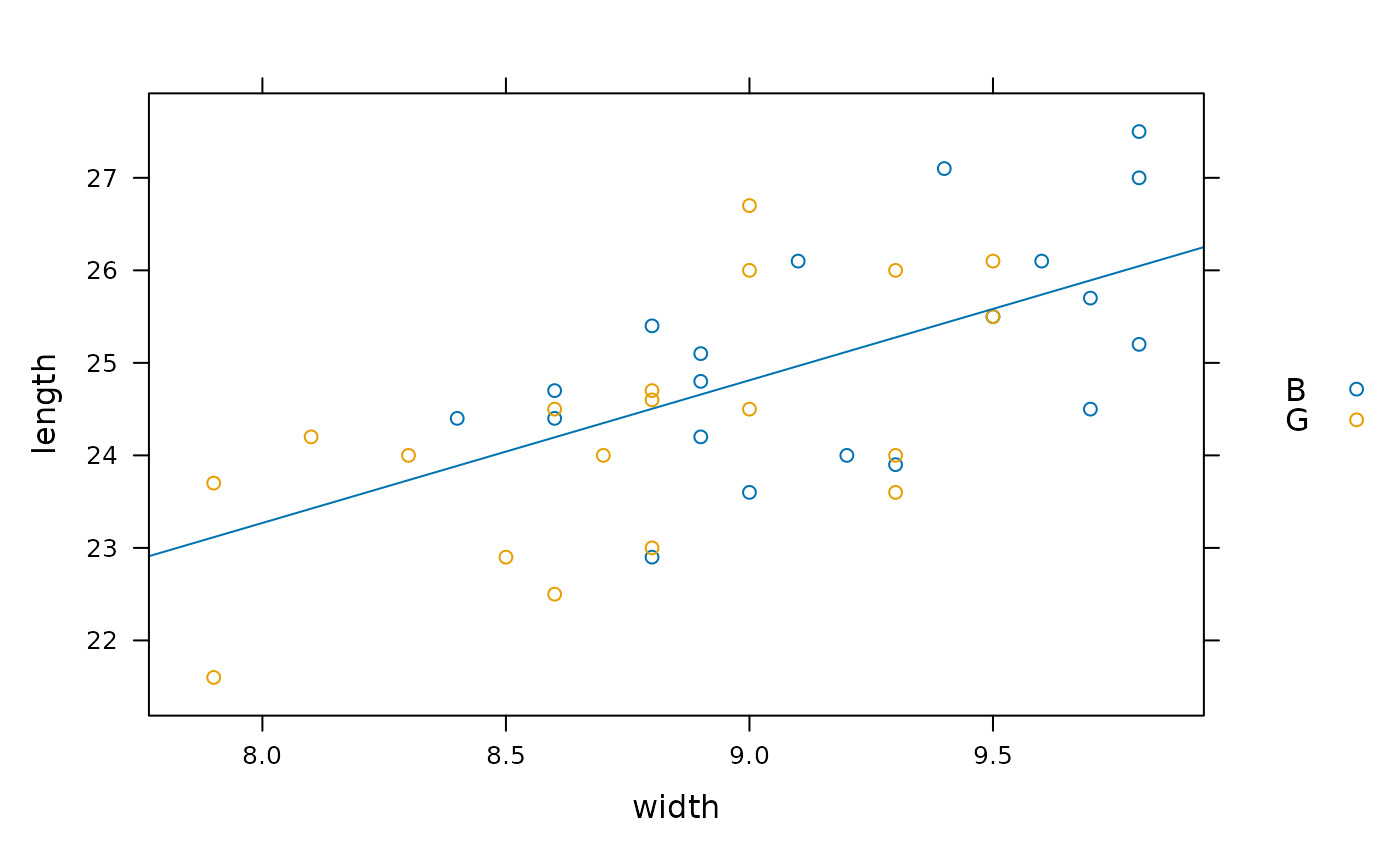
 plotFun(fitted.length(width, sex="B") ~ width, add=TRUE, col=1)
#> converting numerical color value into a color using lattice settings
plotFun(fitted.length(width, sex="B") ~ width, add=TRUE, col=1)
#> converting numerical color value into a color using lattice settings
 plotFun(fitted.length(width, sex="G") ~ width, add=TRUE, col=2)
#> converting numerical color value into a color using lattice settings
#> converting numerical color value into a color using lattice settings
plotFun(fitted.length(width, sex="G") ~ width, add=TRUE, col=2)
#> converting numerical color value into a color using lattice settings
#> converting numerical color value into a color using lattice settings