Less Volume, More Creativity -- Getting Started with the mosaic Package

Project MOSAIC and the `mosaic` package

NSF-funded project to develop a new way to introduce mathematics, statistics, computation and modeling to students in colleges and universities.

more information at mosaic-web.org
the mosaic package is available via
- CRAN
- github
  - updates more frequently than CRAN
  - use devtools::install_github(ProjectMOSAIC/mosaic) to install directly from github
  - add the optional ref = "beta" to install from the beta (developmental) branch
  - add build_vignettes = TRUE if your system is equipped to build vignettes.

A note about this document

This document was originally created as an R presentation to be used as slides accompanying various presentations. It has been converted into a more traditional document for use as a vignette in the mosaic package.

The examples below use the mosaic and mosaicData packages. An earlier version of this document used lattice graphics, but it has been updated to use ggformula

library(mosaic)  # loads mosaicData and ggformula as well

Less Volume, More Creativity

Many of the guiding principles of the mosaic package reflect the “Less Volume, More Creativity” mantra of Mike McCarthy who had a large poster with those words placed in the “war room” (where assistant coaches decide on the game plan for the upcoming opponent) as a constant reminder not to add too much complexity to the game plan.

A lot of times you end up putting in a lot more volume, because you are teaching fundamentals and you are teaching concepts that you need to put in, but you may not necessarily use because they are building blocks for other concepts and variations that will come off of that … In the offseason you have a chance to take a step back and tailor it more specifically towards your team and towards your players.”

Mike McCarthy, former Head Coach, Green Bay Packers

SIBKIS: See It Big, Keep It Simple

Here is another elegant phrasing of a similar principle.

Perfection is achieved, not when there is nothing more to add, but when there is nothing left to take away.

— Antoine de Saint-Exupery (writer, poet, pioneering aviator)

Less Volume, More Creativity in R

One key to successfully introducing R is finding a set of commands that is

small: fewer is better
coherent: commands should be as similar as possible
powerful: can do what needs doing

It is not enough to use R, it must be used elegantly.

Two examples of this principle:

the mosaic package
the dplyr package (Hadley Wickham)

Minimal R

Goal: a minimal set of R commands for Intro Stats

Result: Minimal R Vignette (vignette("MinimalR"))

Much of the work on the mosaic package has been motivated by

The Less Volume, More Creativity approach
The Minimal R goal

A few little details

If you (or your students) are just getting started with R, it is good to keep the following in mind:

R is case sensitive

many students are not case sensitive

Arrows and Tab

up/down arrows scroll through history
TAB completion can simplify typing

If all else fails, try ESC

If you see a + prompt, it means R is waiting for more input
If this is unintentional, you probably have a typo
ESC will get you pack to the command prompt

The Most Important Template

The following template is important because we can do so much with it.

goal ( yyy ~ xxx , data = mydata )

It is useful to name the components of the template:

goal ( y ~ x , data = mydata )

We’re hiding a bit of complexity in the template, and there will be times that we will want to gussy things up a bit. We’ll indicate that by adding ... to the end of the template. Just don’t let ... become a distractor early on.

goal ( y ~ x , data = mydata , …)

Other versions

Here are some variations on the template.

# simpler version
goal(~ x, data = mydata)          
# fancier version
goal(y ~ x | z , data = mydata)   
# unified version
goal(formula, data = mydata)

2 Questions

Using the template generally requires answering two questions. (These questions are useful in the context of nearly all computer tools, just substitute “the computer” in for R in the questions.)

goal ( y ~ x , data = mydata )

What do you want R to do? (goal)

This determines the R function to use

What must R know to do that?

This determines the inputs to the function
Must identify the variables and data frame

How do we make this plot? (Questions)

What is the Goal?

What does R need to know?

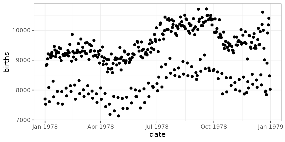
How do we make this plot? (Answers)

What is the Goal?

a scatter plot (gf_point())

What does R need to know?

which variable goes where (births ~ date)
which data set (data = Births78)
- use ?Births78 for documentation

Putting it all together

gf_point(births ~ date, data = Births78)

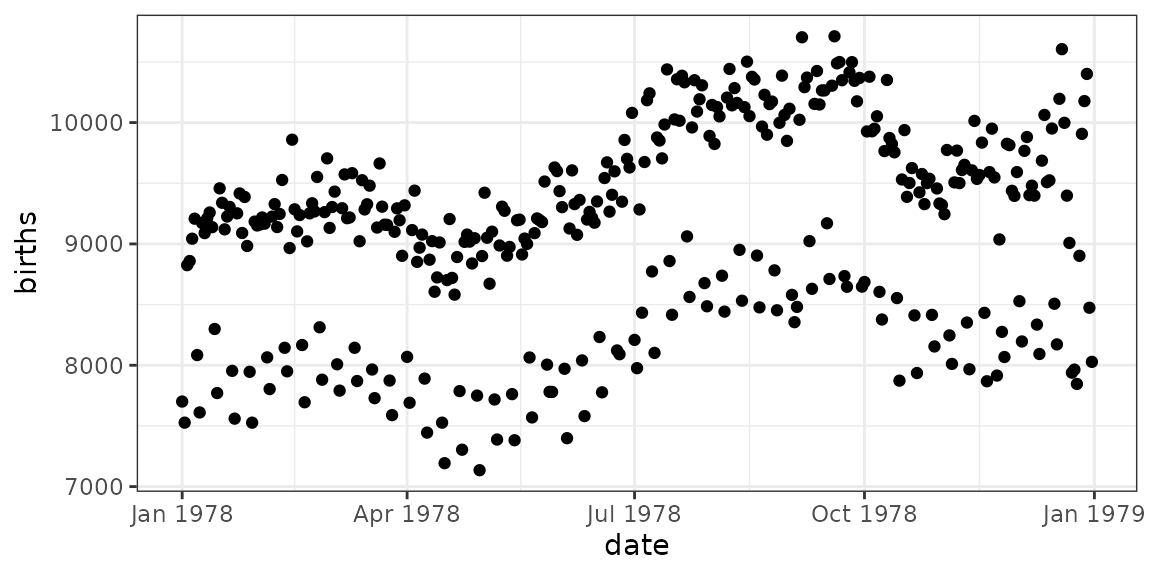
Your turn: How do you make this plot?

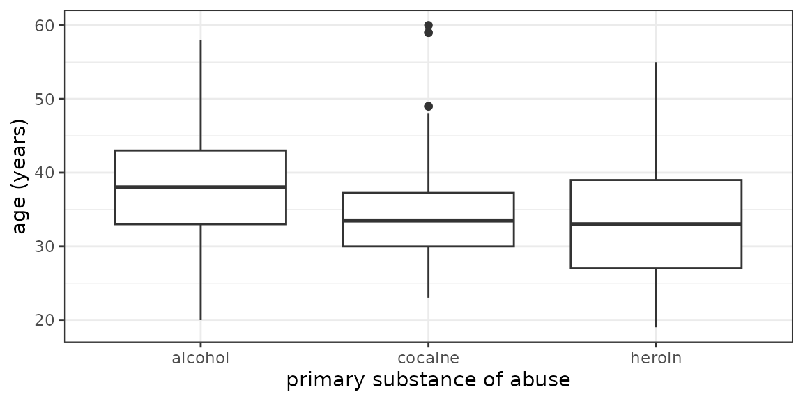
Some things you will need to know:

Command: gf_boxplot()
The data: HELPrct

Variables: age, substance
use ?HELPrct for info about data

Answer

gf_boxplot(age ~ substance, data=HELPrct)

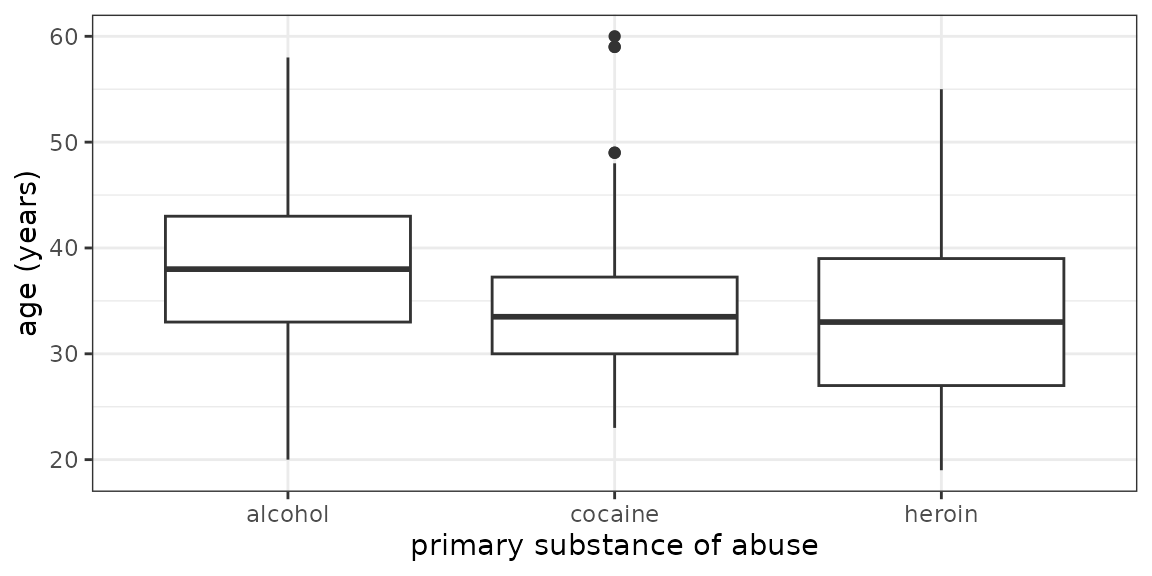
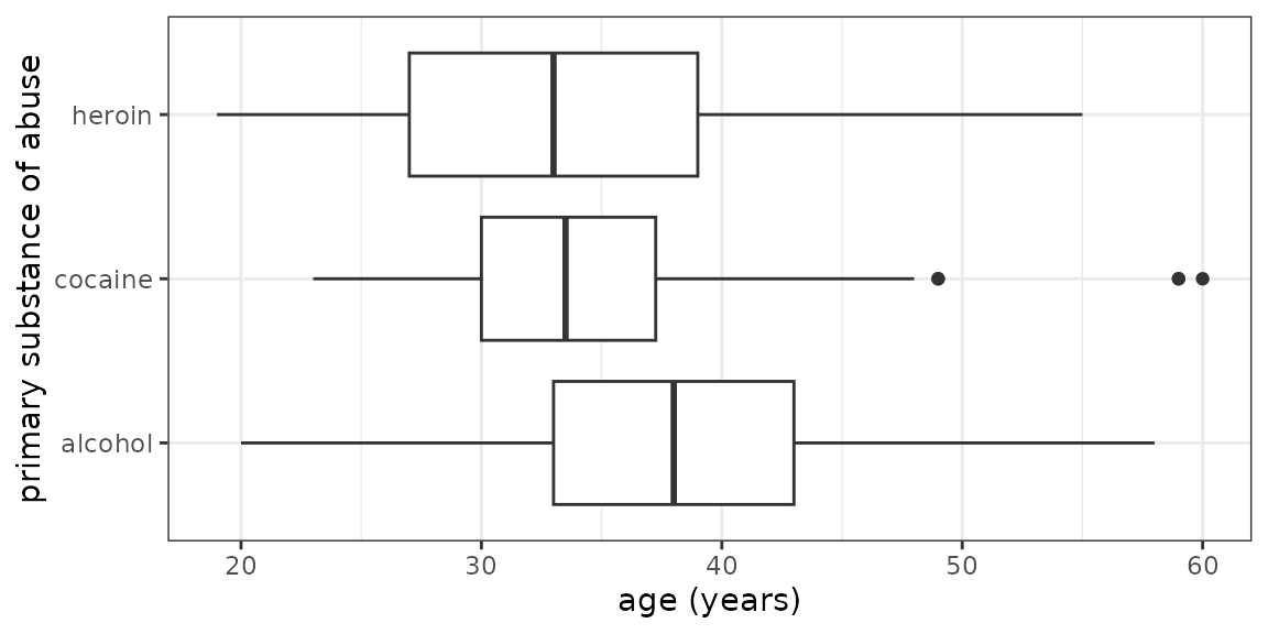
Your turn: How about this one?

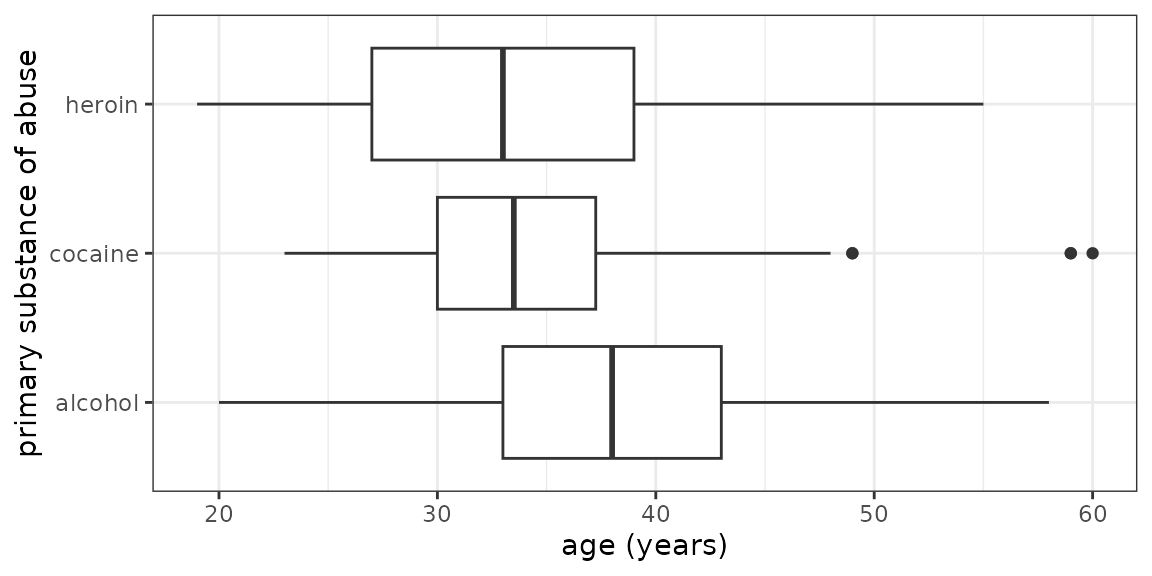
Some things you will need to know:

gf_boxplot() chooses between horizontal and vertical orientation based on the types of variables assigned to each axis.
The data: HELPrct
- Variables: age, substance
- use ?HELPrct for info about data

Answer

gf_boxplot(substance ~ age, data = HELPrct)

Note that we have reversed which variable is mapped to the x-axis and which to the y-axis by reversing their order in the formula.

Graphical Summaries: One Variable

gf_histogram(~ age, data = HELPrct)

## `stat_bin()` using `bins = 30`. Pick better value `binwidth`.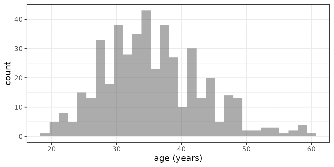

Note: When there is one variable it is on the right side of the formula.

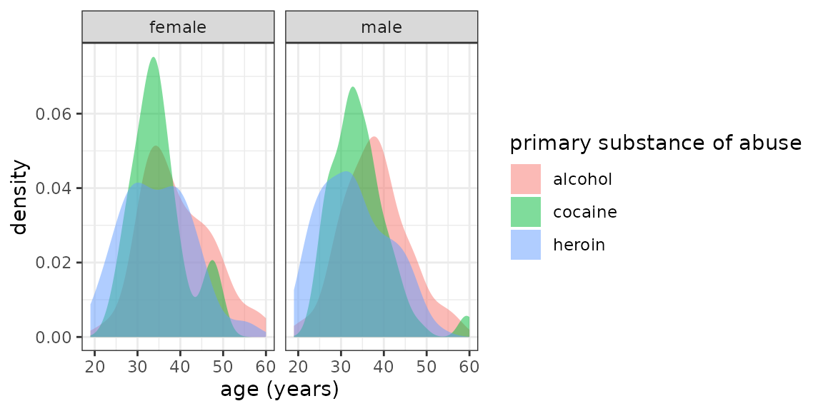
Graphical Summaries: Overview

One Variable

  gf_histogram( ~ age, data = HELPrct) 
    gf_density( ~ age, data = HELPrct) 
    gf_boxplot( ~ age, data = HELPrct) 
         gf_qq( ~ age, data = HELPrct) 
   gf_freqpoly( ~ age, data = HELPrct)

Two Variables

gf_point(i1 ~ age,          data = HELPrct) 
gf_boxplot(age ~ substance, data = HELPrct)

Note: i1 is the average number of drinks (standard units) consumed per day in the past 30 days (measured at baseline)

The Graphics Template

One variable

plotname (

x , data = mydata , …)

gf_histogram(), gf_qq(), gf_density(), gf_freqpoly()

Two Variables

plotname ( y ~ x , data = mydata , …)

gf_point(), gf_line(), gf_boxplot()

Your turn

Create a plot of your own choosing with one of these data sets

names(KidsFeet)    # 4th graders' feet
?KidsFeet

names(Utilities)   # utility bill data
?Utilities

require(NHANES)    # load package
names(NHANES)      # body shape, etc. 
?NHANES

groups and panels

Add color = ~group or fill = ~group to overlay with different colors.
Use y ~ x | z to create multipanel plots.

Here is an example.

gf_density( ~ age | sex, data = HELPrct, fill = ~ substance)

Beginners can create plots with 3 or 4 variables easily and quickly using this template.

Bells & Whistles

The ggformula graphics system includes lots of bells and whistles including

titles
axis labels
colors
sizes
transparency
etc, etc.

I used to introduce these too early. My current approach:

Let the students ask or
Let the data analysis drive

An example with some bells and whistles

library(lubridate)
Births78 <- Births78 %>%
  mutate(weekday = wday(date, label = TRUE, abbr = TRUE))
gf_line(births ~ date, color = ~ weekday, data = Births78)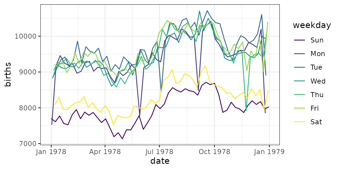

Notes

wday() is in the lubridate package
This version of the plot reveals a clear weekend (and holiday) pattern. Typically, I like to have students conjecture about the “double wave” pattern and see if we can build plots to test their conjectures.

Numerical Summaries

The mosaic package provides functions that make it simple to create numerical summaries using the same template used for graphing (and later for describing linear models).

Numerical Summaries: One Variable

Big idea:

Replace plot name with summary name
Nothing else changes

gf_histogram( ~ age, data = HELPrct)  # binwidth = 5 (or 10) might be good here

## `stat_bin()` using `bins = 30`. Pick better value `binwidth`.

        mean( ~ age, data = HELPrct)

## [1] 35.65342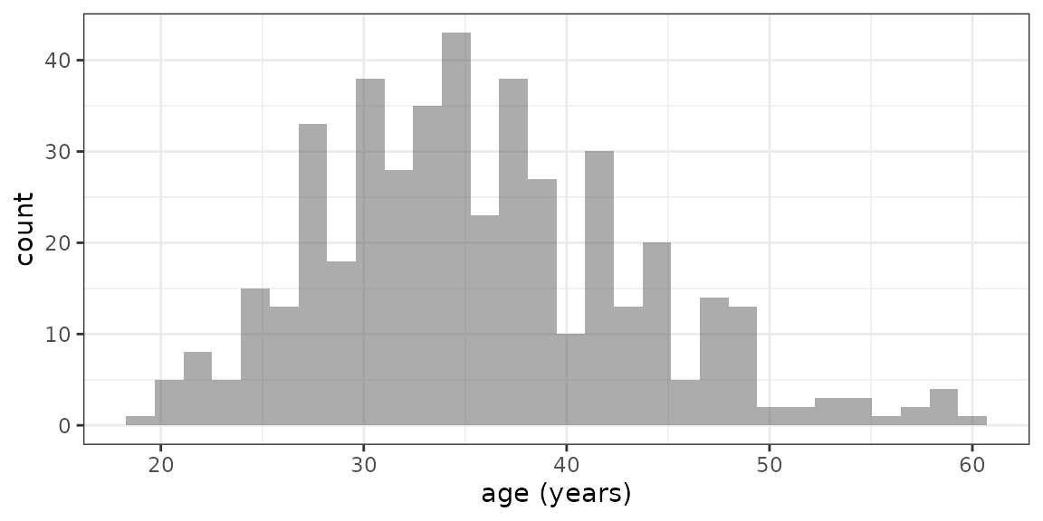

Other summaries

The mosaic package includes formula aware versions of mean(), sd(), var(), min(), max(), sum(), IQR(), …

Also provides favstats() to compute our favorites.

favstats( ~ age, data = HELPrct)

##  min Q1 median Q3 max     mean       sd   n missing
##   19 30     35 40  60 35.65342 7.710266 453       0

favstats() quickly becomes a go-to function in our courses.

df_stats() is similar, but

stores the results in a data frame
can be used to make custom summary tables

df_stats( ~ age, data = HELPrct)

##   response min Q1 median Q3 max     mean       sd   n missing
## 1      age  19 30     35 40  60 35.65342 7.710266 453       0

df_stats( ~ age, data = HELPrct, mean, sd, median, iqr)

##   response     mean       sd median iqr
## 1      age 35.65342 7.710266     35  10

Tallying

tally(~ sex, data = HELPrct)

## sex
## female   male 
##    107    346

tally(~ substance, data = HELPrct)

## substance
## alcohol cocaine  heroin 
##     177     152     124

df_stats(~ substance, data = HELPrct, counts, props)

##    response n_alcohol n_cocaine n_heroin prop_alcohol prop_cocaine prop_heroin
## 1 substance       177       152      124    0.3907285    0.3355408   0.2737307

Numerical Summaries: Two Variables

There are three ways to think about this. All do the same thing.

sd(age ~ substance, data = HELPrct)
sd(~ age | substance, data = HELPrct)
sd(~ age, groups = substance, data = HELPrct)  
# note option color = ~ substance is used for graphics

##  alcohol  cocaine   heroin 
## 7.652272 6.692881 7.986068

This makes it possible to easily convert three different types of plots into the (same) corresponding numerical summary.

df_stats() can also be used with multiple variables and provides a different output format.

df_stats(age ~ substance, data = HELPrct, sd)

##   response substance       sd
## 1      age   alcohol 7.652272
## 2      age   cocaine 6.692881
## 3      age    heroin 7.986068

Numerical Summaries: Tables

2-way tables are just tallies of 2 variables.

tally(sex ~ substance, data = HELPrct)

##         substance
## sex      alcohol cocaine heroin
##   female      36      41     30
##   male       141     111     94

tally( ~ sex + substance, data = HELPrct)

##         substance
## sex      alcohol cocaine heroin
##   female      36      41     30
##   male       141     111     94

df_stats(sex ~ substance, data = HELPrct, counts)

##   response substance n_female n_male
## 1      sex   alcohol       36    141
## 2      sex   cocaine       41    111
## 3      sex    heroin       30     94

Other output formats are available

tally(sex ~ substance,   data = HELPrct, format = "proportion")

##         substance
## sex        alcohol   cocaine    heroin
##   female 0.2033898 0.2697368 0.2419355
##   male   0.7966102 0.7302632 0.7580645

tally(substance ~ sex,   data = HELPrct, format = "proportion", margins = TRUE)

##          sex
## substance    female      male
##   alcohol 0.3364486 0.4075145
##   cocaine 0.3831776 0.3208092
##   heroin  0.2803738 0.2716763
##   Total   1.0000000 1.0000000

tally(~ sex + substance, data = HELPrct, format = "proportion", margins = TRUE)

##         substance
## sex         alcohol    cocaine     heroin      Total
##   female 0.07947020 0.09050773 0.06622517 0.23620309
##   male   0.31125828 0.24503311 0.20750552 0.76379691
##   Total  0.39072848 0.33554084 0.27373068 1.00000000

tally(sex ~ substance,   data = HELPrct, format = "percent")

##         substance
## sex       alcohol  cocaine   heroin
##   female 20.33898 26.97368 24.19355
##   male   79.66102 73.02632 75.80645

df_stats(sex ~ substance,   data = HELPrct, props, percs)

##   response substance prop_female prop_male perc_female perc_male
## 1      sex   alcohol   0.2033898 0.7966102    20.33898  79.66102
## 2      sex   cocaine   0.2697368 0.7302632    26.97368  73.02632
## 3      sex    heroin   0.2419355 0.7580645    24.19355  75.80645

More examples

mean(age ~ substance | sex, data = HELPrct)

##      A.F      C.F      H.F      A.M      C.M      H.M        F        M 
## 39.16667 34.85366 34.66667 37.95035 34.36036 33.05319 36.25234 35.46821

mean(age ~ substance | sex, data = HELPrct, .format = "table")

##   substance sex     mean
## 1         A   F 39.16667
## 2         A   M 37.95035
## 3         C   F 34.85366
## 4         C   M 34.36036
## 5         H   F 34.66667
## 6         H   M 33.05319

I’ve abbreviated some labels to make things fit better. You can do this using mutate() (in the dplyr package) or transform().
This also works for median(), min(), max(), sd(), var(), favstats(), etc.

One Template to Rule a Lot

This master template can be used to do a large portion of what needs doing in an Intro Stats course.

single and multiple variable graphical summaries
single and multiple variable numerical summaries
linear models

      mean(age ~ sex, data = HELPrct)
gf_boxplot(age ~ sex, data = HELPrct) 
        lm(age ~ sex, data = HELPrct)

##   female     male 
## 36.25234 35.46821

## (Intercept)     sexmale 
##  36.2523364  -0.7841284

It can be learned early and practiced often so that students become secure in their ability to use these functions.

Some other things

The mosaic package includes some other things, too

data sets (they have now been moved to separate mosaicData and NHANES packages)
xtras: xchisq.test(), xpnorm(), xqqmath()
- these functions add a bit of extra output to the similarly named functions that don’t have a leading x
mplot()
- mplot(HELPrct) interactive plot creation
- replacements for plot() in some situations
simplified gf_histogram() controls (e.g., binwidth)
simplified ways to add onto lattice plots (gf_refine())

Examples

xpnorm(700, mean = 500, sd = 100)

##

## If X ~ N(500, 100), then

##  P(X <= 700) = P(Z <= 2) = 0.9772

##  P(X >  700) = P(Z >  2) = 0.02275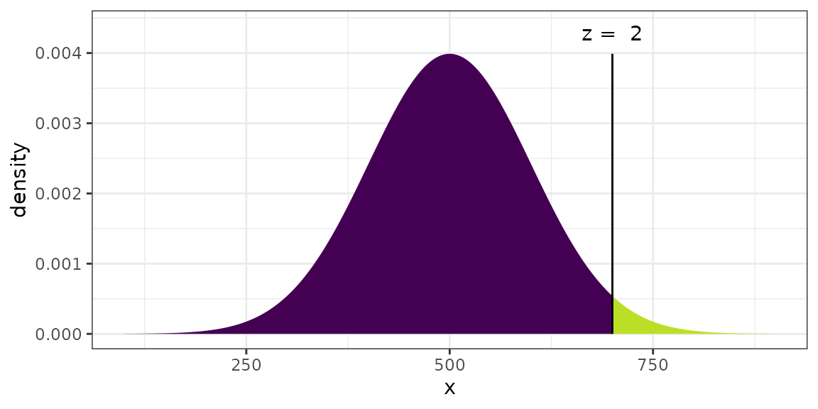

##

## [1] 0.9772499

xpnorm(c(300, 700), mean = 500, sd = 100)

##

## If X ~ N(500, 100), then

##  P(X <= 300) = P(Z <= -2) = 0.02275  P(X <= 700) = P(Z <=  2) = 0.97725

##  P(X >  300) = P(Z >  -2) = 0.97725  P(X >  700) = P(Z >   2) = 0.02275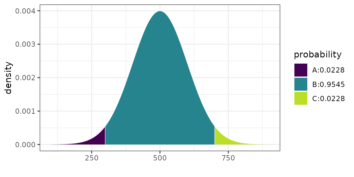

##

## [1] 0.02275013 0.97724987

xchisq.test(phs)

## 
##  Pearson's Chi-squared test with Yates' continuity correction
## 
## data:  x
## X-squared = 24.429, df = 1, p-value = 7.71e-07
## 
##    104.00   10933.00 
## (  146.52) (10890.48)
## [12.05]  [ 0.16] 
## <-3.51>  < 0.41> 
##    
##    189.00   10845.00 
## (  146.48) (10887.52)
## [12.05]  [ 0.16] 
## < 3.51>  <-0.41> 
##    
## key:
##  observed
##  (expected)
##  [contribution to X-squared]
##  <Pearson residual>

Modeling

Modeling is really the starting point for the mosaic design.

linear models (lm() and glm()) defined the template
lattice graphics use the template (so we chose lattice)
we added functionality so numerical summaries can be done with the same template
additional things added to make modeling easier for beginners

Models as Functions

model <- lm(width ~ length * sex, 
            data = KidsFeet)
Width <- makeFun(model)
Width(length = 25, sex = "B")

##        1 
## 9.167675

Width(length = 25, sex = "G")

##        1 
## 8.939312

Once models have been converted into functions, we can easily add them to our plots using plotFun().

gf_point(width ~ length, data = KidsFeet, 
        color = ~ sex) %>%
  gf_fun(Width(length, sex = "B") ~ length, color = ~"B") %>%
  gf_fun(Width(length, sex = "G") ~ length, color = ~"G")

## Warning in stat_function(geom = "path", position = "identity", mapping = structure(list(: All aesthetics have length 1, but the data has 39 rows.
## ℹ Please consider using `annotate()` or provide this layer with data containing a single
##   row.

## Warning in stat_function(geom = "path", position = "identity", mapping = structure(list(: All aesthetics have length 1, but the data has 39 rows.
## ℹ Please consider using `annotate()` or provide this layer with data containing a single
##   row.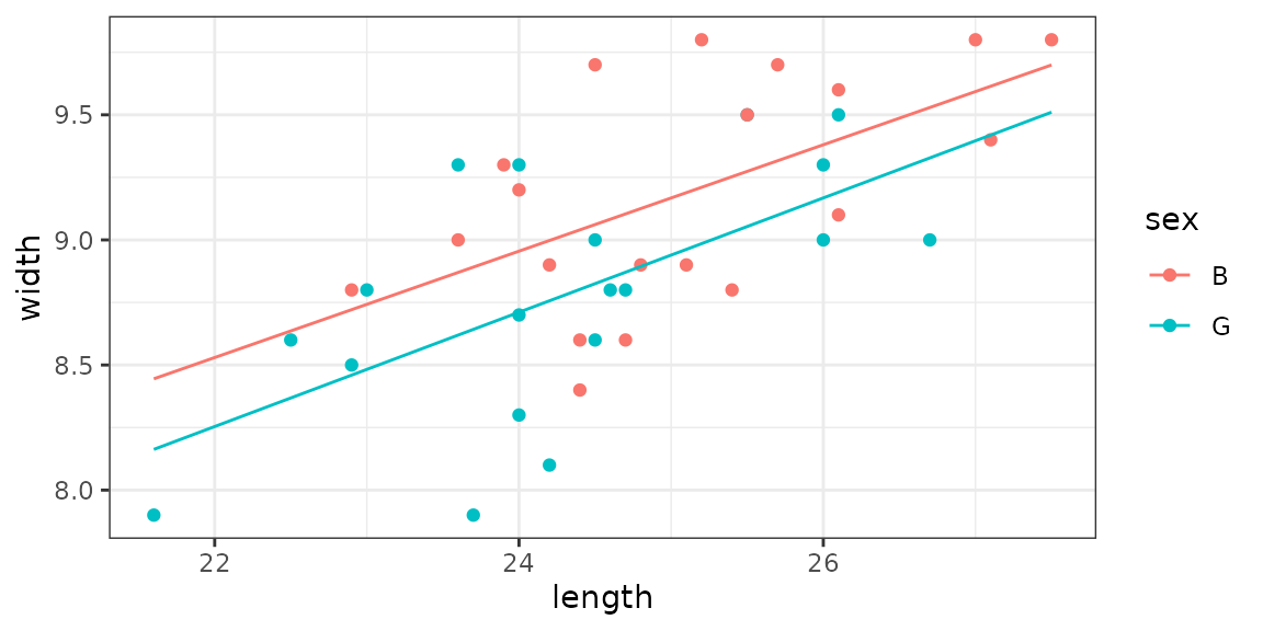

Resampling – You can do() it!

If you want to teach using randomization tests and bootstrap intervals, the mosaic package provides some functions to simplify creating the random distirubtions involved.

An example: The Lady Tasting Tea

Often used on first day of class
Story
- woman claims she can tell whether milk has been poured into tea or vice versa.
- Question: How do we test this claim?

We use rflip() to simulate flipping coins

rflip()

## 
## Flipping 1 coin [ Prob(Heads) = 0.5 ] ...
## 
## H
## 
## Number of Heads: 1 [Proportion Heads: 1]

Note: We do this with students who do not (yet) know what a binomial distribution is, so we want to avoid using rbinom() at this point.

Rather than flip each coin separately, we can flip multiple coins at once.

rflip(10)

## 
## Flipping 10 coins [ Prob(Heads) = 0.5 ] ...
## 
## H H H T T T H H H T
## 
## Number of Heads: 6 [Proportion Heads: 0.6]

easier to consider heads = correct; tails = incorrect than to compare with a given pattern
- this switch bothers me more than it bothers my students

Now let’s do that a lot of times

rflip(10) simulates 1 lady tasting 10 cups 1 time.

We can do that many times to see how guessing ladies do:

do(2) * rflip(10)

##    n heads tails prop
## 1 10     6     4  0.6
## 2 10     5     5  0.5

do() is clever about what it remembers (in many common situations)
2 isn’t many – we’ll do many next – but it is a good idea to take a look at a small example before generating a lot of random data.

Now let’s simulate 5000 guessing ladies

Ladies <- do(5000) * rflip(10)
head(Ladies, 2)

##    n heads tails prop
## 1 10     4     6  0.4
## 2 10     7     3  0.7

gf_histogram(~ heads, data = Ladies, binwidth = 1)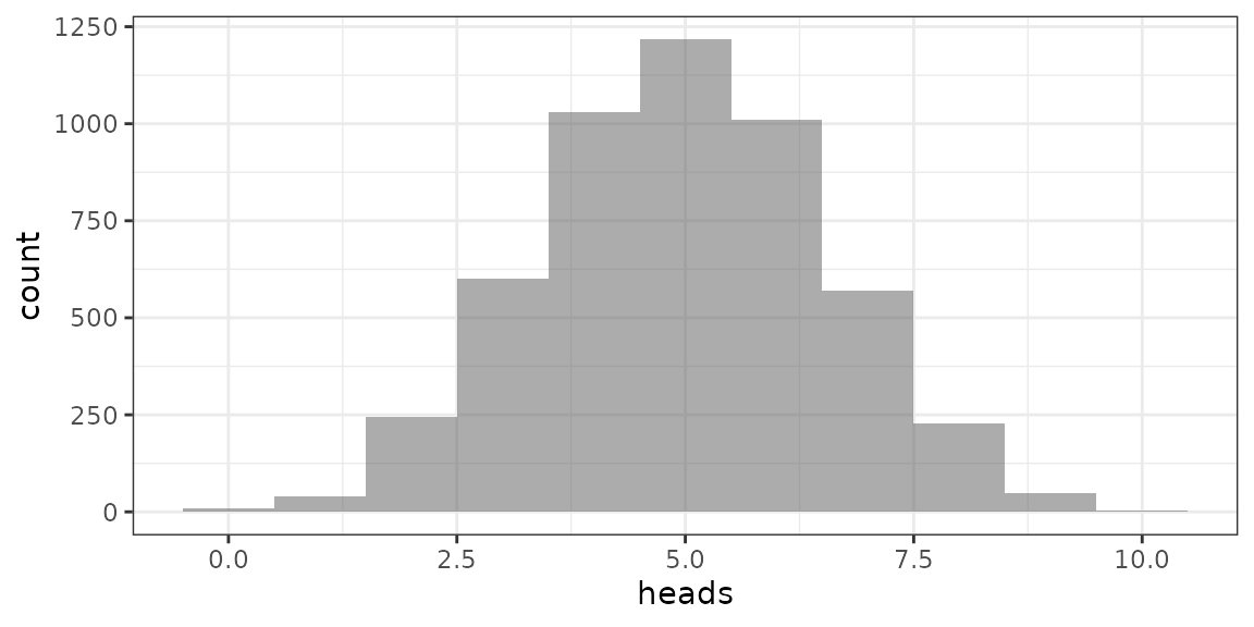

Q. How often does guessing score 9 or 10?

Here are 3 ways to find out

tally( ~ (heads >= 9), data = Ladies)

## (heads >= 9)
##  TRUE FALSE 
##    52  4948

tally( ~ (heads >= 9), data = Ladies, format = "prop")

## (heads >= 9)
##   TRUE  FALSE 
## 0.0104 0.9896

 prop( ~ (heads >= 9), data = Ladies)

## prop_TRUE 
##    0.0104

A general approach to randomization

The Lady Tasting Tea illustrates a 3-step process that can be reused in many situations:

Do it for your data
Do it for “random” data
Do it lots of times for “random” data

definition of “random” is important, but can often be handled by the mosaic functions shuffle() or resample()

Example: Do mean ages differ by sex?

diffmean(age ~ sex, data = HELPrct)

##   diffmean 
## -0.7841284

do(1) * 
  diffmean(age ~ shuffle(sex), data = HELPrct)

##     diffmean
## 1 0.09686133

Null <- do(5000) * 
  diffmean(age ~ shuffle(sex), data = HELPrct)

prop( ~ (abs(diffmean) > 0.7841), data = Null)

## prop_TRUE 
##    0.3412

gf_histogram( ~ diffmean, data = Null) %>%
  gf_vline(xintercept = -0.7841)

## `stat_bin()` using `bins = 30`. Pick better value `binwidth`.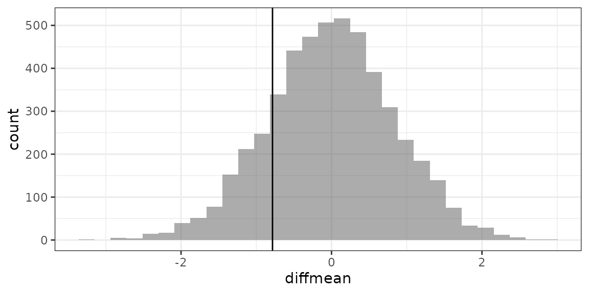

Example: Bootstrap CI for difference in means

Bootstrap <- do(5000) * 
  diffmean(age ~ sex, data = resample(HELPrct))

gf_histogram( ~ diffmean, data = Bootstrap) %>%
  gf_vline(xintercept = -0.7841)

## `stat_bin()` using `bins = 30`. Pick better value `binwidth`.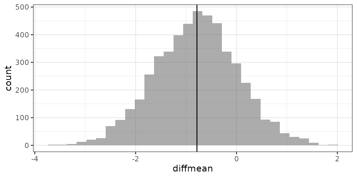

cdata( ~ diffmean, data = Bootstrap, p = 0.95)

##          lower     upper central.p
## 2.5% -2.438299 0.8177243      0.95

confint(Bootstrap, method = "quantile")

##       name     lower     upper level     method   estimate
## 1 diffmean -2.438299 0.8177243  0.95 percentile -0.7841284

confint(Bootstrap)  # default uses bootstrap st. err.

##       name     lower     upper level     method   estimate
## 1 diffmean -2.438299 0.8177243  0.95 percentile -0.7841284

Randomization and linear models

do(1) * lm(width ~ length, data = KidsFeet)

##   Intercept    length     sigma r.squared        F numdf dendf .row .index
## 1  2.862276 0.2479478 0.3963356 0.4110041 25.81878     1    37    1      1

do(3) * lm(width ~ shuffle(length), data = KidsFeet)

##   Intercept      length     sigma   r.squared         F numdf dendf .row .index
## 1  6.347607  0.10697295 0.4962778 0.076502169 3.0650643     1    37    1      1
## 2  9.877910 -0.03582090 0.5142048 0.008578250 0.3201415     1    37    1      2
## 3  9.840434 -0.03430504 0.5143891 0.007867588 0.2934092     1    37    1      3

do(1) * 
  lm(width ~ length + sex, data = KidsFeet)

##   Intercept   length       sexG     sigma r.squared        F numdf dendf .row .index
## 1  3.641168 0.221025 -0.2325175 0.3848905 0.4595428 15.30513     2    36    1      1

do(3) * 
  lm(width ~ length + shuffle(sex), data = KidsFeet)

##   Intercept    length        sexG     sigma r.squared        F numdf dendf .row .index
## 1  3.068833 0.2378303  0.08945102 0.3993335 0.4182207 12.93957     2    36    1      1
## 2  2.916037 0.2478853 -0.10717940 0.3979148 0.4223471 13.16058     2    36    1      2
## 3  3.351286 0.2334825 -0.26968267 0.3770203 0.4814193 16.71013     2    36    1      3

Null <- do(5000) * 
  lm(width ~ length + shuffle(sex), 
                       data = KidsFeet)
gf_histogram( ~ sexG, data = Null, boundary = -0.2325) %>%
  gf_vline(xintercept = -0.2325)

## `stat_bin()` using `bins = 30`. Pick better value `binwidth`.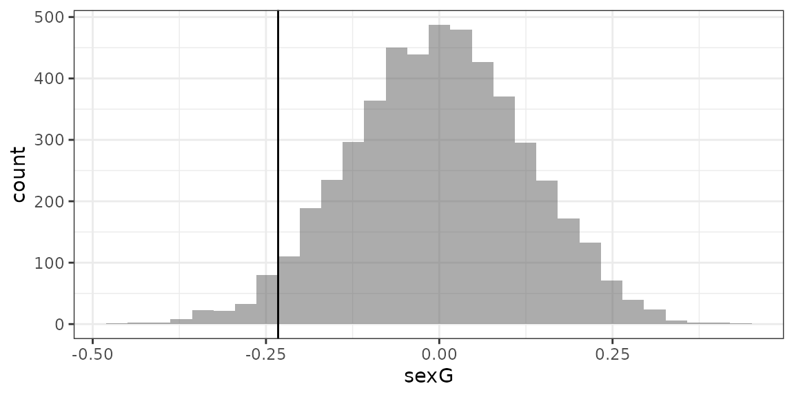

gf_histogram(~ sexG, data = Null, boundary = -0.2325) %>%
  gf_vline(xintercept = -0.2325)

## `stat_bin()` using `bins = 30`. Pick better value `binwidth`.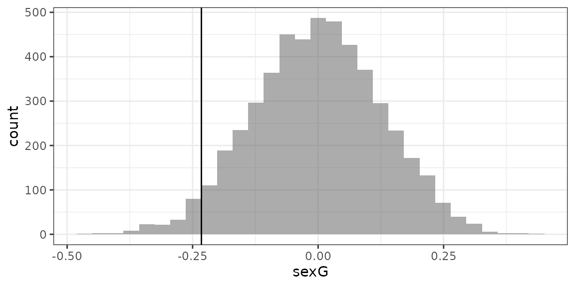

prop(~ (sexG <= -0.2325), data = Null)

## prop_TRUE 
##    0.0344

Want to learn more?

More mosaic resources can be found at https://www.mosaic-web.org/mosaic/articles/mosaic-resources.html.

The RJournal paper entitled “mosaic Package: Helping Students to `Think with Data’ Using R (https://journal.r-project.org/articles/RJ-2017-024/index.html) provides further discussion of the mosaic modeling language and approach to teaching.

Randall Pruim (updated by Nicholas Horton)

2026-06-04

Project MOSAIC and the mosaic package

A note about this document

Less Volume, More Creativity

SIBKIS: See It Big, Keep It Simple

Less Volume, More Creativity in R

Minimal R

A few little details

R is case sensitive

Arrows and Tab

If all else fails, try ESC

The Most Important Template

goal ( yyy ~ xxx , data = mydata )

goal ( y ~ x , data = mydata )

goal ( y ~ x , data = mydata , …)

Other versions

2 Questions

goal ( y ~ x , data = mydata )

What do you want R to do? (goal)

What must R know to do that?

How do we make this plot? (Questions)

What is the Goal?

What does R need to know?

How do we make this plot? (Answers)

What is the Goal?

What does R need to know?

Putting it all together

Your turn: How do you make this plot?

Answer

Your turn: How about this one?

Answer

Graphical Summaries: One Variable

Graphical Summaries: Overview

One Variable

Two Variables

The Graphics Template

One variable

plotname ( x , data = mydata , …)

Two Variables

plotname ( y ~ x , data = mydata , …)

Your turn

groups and panels

Bells & Whistles

An example with some bells and whistles

Numerical Summaries

Numerical Summaries: One Variable

Other summaries

Tallying

Numerical Summaries: Two Variables

Numerical Summaries: Tables

More examples

One Template to Rule a Lot

Some other things

Examples

Modeling

Models as Functions

Resampling – You can do() it!

An example: The Lady Tasting Tea

Now let’s do that a lot of times

A general approach to randomization

Example: Do mean ages differ by sex?

Example: Bootstrap CI for difference in means

Randomization and linear models

Want to learn more?

Project MOSAIC and the `mosaic` package

plotname (

x , data = mydata , …)