Tally test statistics from data and from multiple draws from a simulated null distribution
Usage
statTally(
  sample,
  rdata,
  FUN,
  direction = NULL,
  alternative = c("default", "two.sided", "less", "greater"),
  sig.level = 0.1,
  system = c("gg", "lattice"),
  shade = "navy",
  alpha = 0.1,
  binwidth = NULL,
  bins = NULL,
  fill = "gray80",
  color = "black",
  center = NULL,
  stemplot = dim(rdata)[direction] < 201,
  q = c(0.5, 0.9, 0.95, 0.99),
  fun = function(x) x,
  xlim,
  quiet = FALSE,
  ...
)
Arguments
- sample
sample data
- rdata
a matrix of randomly generated data under null hypothesis.
- FUN
a function that computes the test statistic from a data set. The default value does nothing, making it easy to use this to tabulate precomputed statistics into a null distribution. See the examples.
- direction
1 or 2 indicating whether samples in
rdataare in rows (1) or columns (2).- alternative
one of
default,two.sided,less, orgreater- sig.level
significance threshold for
wilcox.testused to detect lack of symmetry- system
graphics system to use for the plot
- shade
a color to use for shading.
- alpha
opacity of shading.
- binwidth
bin width for histogram.
- bins
number of bins for histogram.
- fill
fill color for histogram.
- color
border color for histogram.
- center
center of null distribution
- stemplot
indicates whether a stem plot should be displayed
- q
quantiles of sampling distribution to display
- fun
same as
FUNso you don't have to remember if it should be capitalized- xlim
limits for the horizontal axis of the plot.
- quiet
a logicial indicating whether the text output should be suppressed
- ...
additional arguments passed to
lattice::histogram()orggplot2::geom_histogram()
Value
A lattice or ggplot showing the sampling distribution.
As side effects, information about the empirical sampling distribution and (optionally) a stem plot are printed to the screen.
Examples
# is my spinner fair?
x <- c(10, 18, 9, 15) # counts in four cells
rdata <- rmultinom(999, sum(x), prob = rep(.25, 4))
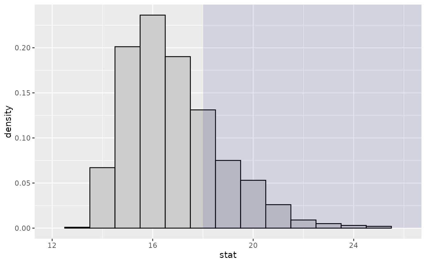
statTally(x, rdata, fun = max, binwidth = 1) # unusual test statistic
#>
#> Null distribution appears to be asymmetric. (p = 0)
#>
#> Test statistic applied to sample data = 18
#>
#> Quantiles of test statistic applied to random data:
#> 50% 90% 95% 99%
#> 16.00 19.00 20.00 22.02
#>
#> Of the 1000 samples (1 original + 999 random),
#> 132 ( 13.2 % ) had test stats = 18
#> 305 ( 30.5 % ) had test stats >= 18
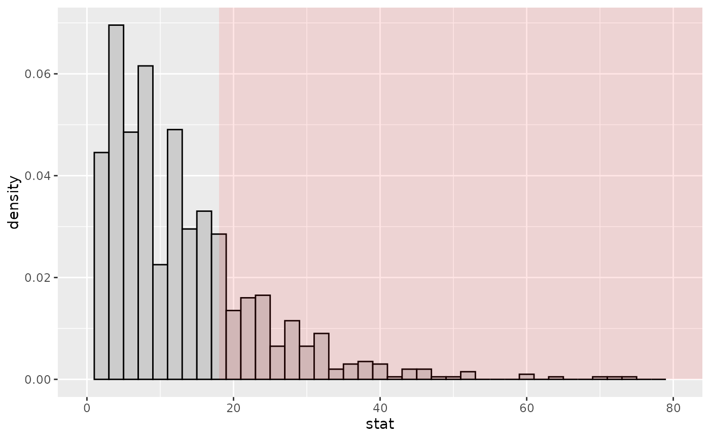
 statTally(x, rdata, fun = var, shade = "red", binwidth = 2) # equivalent to chi-squared test
#>
#> Null distribution appears to be asymmetric. (p = 9.63e-08)
#>
#> Test statistic applied to sample data = 18
#>
#> Quantiles of test statistic applied to random data:
#> 50% 90% 95% 99%
#> 10.00000 26.00000 32.66667 48.70667
#>
#> Of the 1000 samples (1 original + 999 random),
#> 39 ( 3.9 % ) had test stats = 18
#> 255 ( 25.5 % ) had test stats >= 18
statTally(x, rdata, fun = var, shade = "red", binwidth = 2) # equivalent to chi-squared test
#>
#> Null distribution appears to be asymmetric. (p = 9.63e-08)
#>
#> Test statistic applied to sample data = 18
#>
#> Quantiles of test statistic applied to random data:
#> 50% 90% 95% 99%
#> 10.00000 26.00000 32.66667 48.70667
#>
#> Of the 1000 samples (1 original + 999 random),
#> 39 ( 3.9 % ) had test stats = 18
#> 255 ( 25.5 % ) had test stats >= 18
 # Can also be used with test stats that are precomputed.
if (require(mosaicData)) {
D <- diffmean( age ~ sex, data = HELPrct); D
nullDist <- do(999) * diffmean( age ~ shuffle(sex), data = HELPrct)
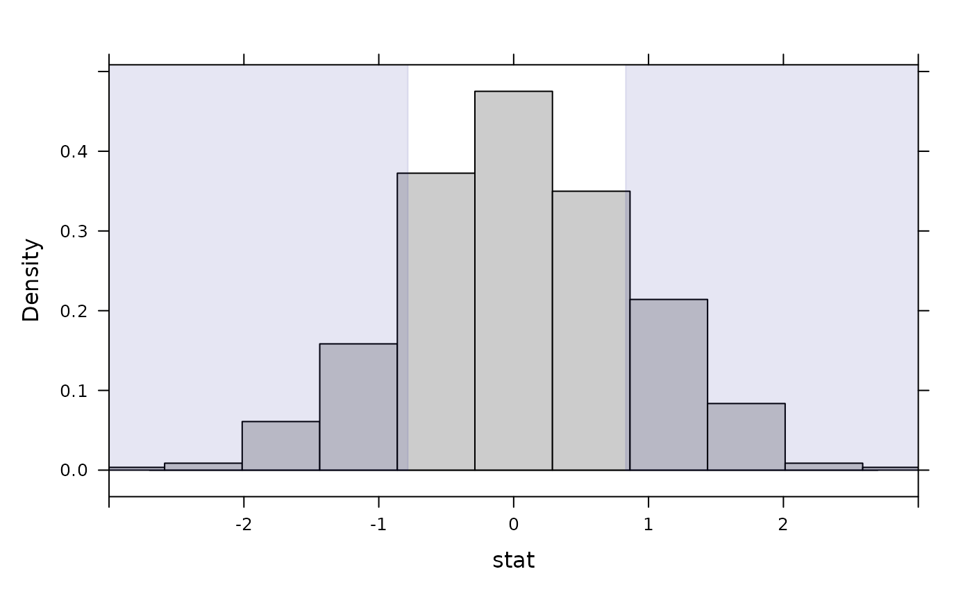
statTally(D, nullDist)
statTally(D, nullDist, system = "lattice")
}
#>
#> Null distribution appears to be symmetric. (p = 0.338 )
#>
#> Test statistic applied to sample data = -0.7841
#>
#> Quantiles of test statistic applied to random data:
#> 50% 90% 95% 99%
#> 0.02344552 1.17362649 1.47952569 1.95770731
#>
#> Of the 1000 samples (1 original + 999 random),
#> 6 ( 0.6 % ) had test stats = -0.7841
#> 155 ( 15.5 % ) had test stats <= -0.7841
#> 185 ( 18.5 % ) had test stats >= 0.831
#>
#> Null distribution appears to be symmetric. (p = 0.338 )
#>
#> Test statistic applied to sample data = -0.7841
#>
#> Quantiles of test statistic applied to random data:
#> 50% 90% 95% 99%
#> 0.02344552 1.17362649 1.47952569 1.95770731
#>
#> Of the 1000 samples (1 original + 999 random),
#> 6 ( 0.6 % ) had test stats = -0.7841
#> 155 ( 15.5 % ) had test stats <= -0.7841
#> 185 ( 18.5 % ) had test stats >= 0.831
# Can also be used with test stats that are precomputed.
if (require(mosaicData)) {
D <- diffmean( age ~ sex, data = HELPrct); D
nullDist <- do(999) * diffmean( age ~ shuffle(sex), data = HELPrct)
statTally(D, nullDist)
statTally(D, nullDist, system = "lattice")
}
#>
#> Null distribution appears to be symmetric. (p = 0.338 )
#>
#> Test statistic applied to sample data = -0.7841
#>
#> Quantiles of test statistic applied to random data:
#> 50% 90% 95% 99%
#> 0.02344552 1.17362649 1.47952569 1.95770731
#>
#> Of the 1000 samples (1 original + 999 random),
#> 6 ( 0.6 % ) had test stats = -0.7841
#> 155 ( 15.5 % ) had test stats <= -0.7841
#> 185 ( 18.5 % ) had test stats >= 0.831
#>
#> Null distribution appears to be symmetric. (p = 0.338 )
#>
#> Test statistic applied to sample data = -0.7841
#>
#> Quantiles of test statistic applied to random data:
#> 50% 90% 95% 99%
#> 0.02344552 1.17362649 1.47952569 1.95770731
#>
#> Of the 1000 samples (1 original + 999 random),
#> 6 ( 0.6 % ) had test stats = -0.7841
#> 155 ( 15.5 % ) had test stats <= -0.7841
#> 185 ( 18.5 % ) had test stats >= 0.831