Capturing evaluation information with evals

evals is aimed at collecting as much information as possible while evaluating R code. It can evaluate a character vector of R expressions, and it returns a list of information captured while running them:

src holds the R expression,
result contains the raw R object as-is,
output represents how the R object is printed to the standard output,
type is the class of the returned R object,
msg is a list of messages captured while evaluating the R expression. Among other messages, warnings/errors will appear here.
stdout contains what, if anything, was written to the standard output.

Besides capturing evaluation information, evals is able to automatically identify whether an R expression is returning anything to a graphical device, and can save the resulting image in a variety of file formats.

Another interesting evals feature is caching the results of evaluated expressions. Read the caching section for more details.

evals has a large number of options, which allow users to customize the call exactly as needed. Here we will focus on the most useful features, but the full list of options, with explanations, can be viewed by calling ?evalsOptions. Also evals support permanent options that will persist for all calls to evals, this can be achieved by calling evalsOptions.

Let’s start with a basic example by evaluating 1:10 and collecting all information about it:

evals('1:10')
#> [[1]]
#> $src
#> [1] "1:10"
#> 
#> $result
#>  [1]  1  2  3  4  5  6  7  8  9 10
#> 
#> $output
#> [1] " [1]  1  2  3  4  5  6  7  8  9 10"
#> 
#> $type
#> [1] "integer"
#> 
#> $msg
#> $msg$messages
#> NULL
#> 
#> $msg$warnings
#> NULL
#> 
#> $msg$errors
#> NULL
#> 
#> 
#> $stdout
#> NULL
#> 
#> attr(,"class")
#> [1] "evals"

Not all the information might be useful, so evals makes it is possible to capture only some of the information, by specifying the output parameter:

evals('1:10', output = c('result', 'output'))
#> [[1]]
#> $result
#>  [1]  1  2  3  4  5  6  7  8  9 10
#> 
#> $output
#> [1] " [1]  1  2  3  4  5  6  7  8  9 10"
#> 
#> attr(,"class")
#> [1] "evals"

One of the neat features of evals that it catches errors/warnings without interrupting the evaluation and saves them.

evals('x')[[1]]$msg
#> $messages
#> NULL
#> 
#> $warnings
#> NULL
#> 
#> $errors
#> [1] "object 'x' not found"
evals('as.numeric("1.1a")')[[1]]$msg
#> $messages
#> NULL
#> 
#> $warnings
#> [1] "NAs introduced by coercion"
#> 
#> $errors
#> NULL

Graphs and Graphical Options

As mentioned before, evals captures the output to graphical devices and saves it:

evals('plot(mtcars)')[[1]]$result
#> [1] "my_plots/test.jpeg"
#> attr(,"class")
#> [1] "image"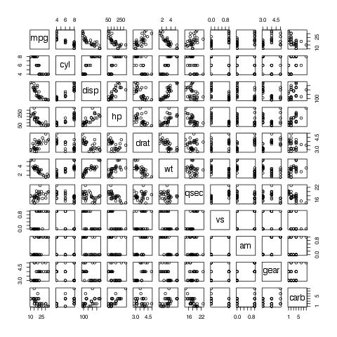

You can specify the output directory using the graph.dir parameter, and the output type using the graph.output parameter. Currently, it could be any of grDevices: png, bmp,jpeg,jpg, tiff, svg, or pdf.

evals('plot(mtcars)', graph.dir = 'my_plots', graph.output = 'jpg')[[1]]$result
#> [1] "my_plots/test.jpeg"
#> attr(,"class")
#> [1] "image"

Moreover, evals provides facilities to:

save the environments in which plots were generated
save the plot via recordPlot to distinct files with recodplot extension
save the raw R object returned (usually with lattice or ggplot2) while generating the plot to distinct files with RDS extension

Style unification

evals provides very powerful facilities to unify the styling of images produced by different packages, like ggplot2 and lattice.

Let’s prepare the data for plotting:

## generating dataset
set.seed(1)
df <- mtcars[, c('hp', 'wt')]
df$factor <- sample(c('Foo', 'Bar', 'Foo bar'), size = nrow(df), replace = TRUE)
df$factor2 <- sample(c('Foo', 'Bar', 'Foo bar'), size = nrow(df), replace = TRUE)
df$time <- 1:nrow(df)

Now let’s plot the histograms:

evalsOptions('graph.unify', TRUE)
evals('histogram(df$hp, main = "Histogram with lattice")')[[1]]$result
#> [1] "my_plots/test.jpeg"
#> attr(,"class")
#> [1] "image"
evals('ggplot(df) + geom_histogram(aes(x = hp), binwidth = 50) + ggtitle("Histogram with ggplot2")')[[1]]$result
#> Warning: The `size` argument of `element_line()` is deprecated as of ggplot2 3.4.0.
#> ℹ Please use the `linewidth` argument instead.
#> ℹ The deprecated feature was likely used in the pander package.
#>   Please report the issue at <https://github.com/rapporter/pander/issues>.
#> This warning is displayed once per session.
#> Call `lifecycle::last_lifecycle_warnings()` to see where this warning was
#> generated.
#> [1] "my_plots/test.jpeg"
#> attr(,"class")
#> [1] "image"
evalsOptions('graph.unify', FALSE)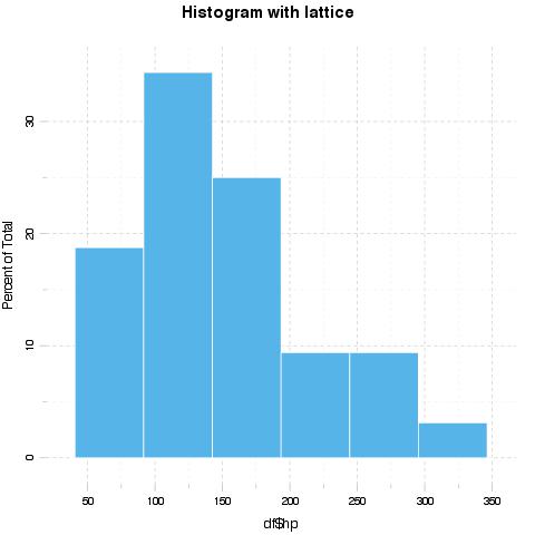

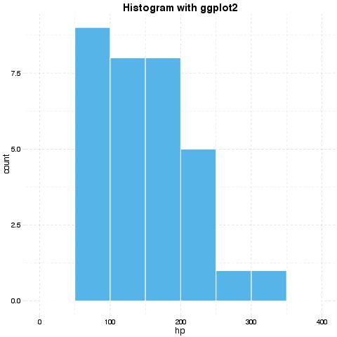
Options for unification can be set with panderOptions. For example:

panderOptions('graph.fontfamily', "Comic Sans MS")
panderOptions('graph.fontsize', 18)
panderOptions('graph.fontcolor', 'blue')
panderOptions('graph.grid.color', 'blue')
panderOptions('graph.axis.angle', 3)
panderOptions('graph.boxes', T)
panderOptions('graph.legend.position', 'top')
panderOptions('graph.colors', rainbow(5))
panderOptions('graph.grid', FALSE)
panderOptions('graph.symbol', 22)

More information and examples on style unification can be obtained by Pandoc.brewing the tutorial available here.

Logging

To make execution and debugging easier to understand, evals provides logging with the log parameter. Logging in evals relies on the logger package, which provides a logging API similar to log4j. Basic example:

x <- evals('1:10', log = 'foo')
#> INFO [2026-02-04 01:45:24] Command run: 1:10

logger’s thresholds range from most verbose to least verbose: TRACE, DEBUG, INFO, WARN, ERROR, FATAL. The threshold defaults to INFO, which will hide some unessential information. To permanently set the threshold for logger use log_threshold:

evalsOptions('log', 'evals')
log_threshold(TRACE, namespace = 'evals')
x <- evals('1:10', cache.time = 0)
#> INFO [2026-02-04 01:45:24] Command run: 1:10
#> TRACE [2026-02-04 01:45:24] Cached result
#> DEBUG [2026-02-04 01:45:24] Returned object: class = integer, length = 10, dim = , size = 96 bytes

logger also provides a very useful ability to write logs to files instead of printing them to the prompt:

t <- tempfile()
log_appender(appender_file(t), namespace = 'evals')
x <- evals('1:10', log = 'evals')
readLines(t)
#> [1] "INFO [2026-02-04 01:45:24] Command run: 1:10"          
#> [2] "TRACE [2026-02-04 01:45:24] Returning cached R object."
# revert back to console
log_appender(appender_stdout, namespace = 'evals')

Result Caching

evals is uses a custom caching algorithm to cache the results of evaluated R expressions.

How it works

All R code passed to evals is split into single expressions and parsed.
For each R expression (function call, assignment, etc.), evals extracts symbols in a separate list in getCallParts. This list describes the unique structure and the content of the passed R expressions
A hash is computed for each list element and cached in pander’s local environments. This is useful if you are using large data frames; otherwise, the caching algorithm would have to compute the hash for the same data frame each time it’s touched! This way the hash is recomputed only if the R object with the given name is changed.
The list of such R objects is serialized, then an SHA-1 hash is computed, taking into consideration panderOptions and evalsOptions, which all together is unique and there is no real risk of collision.
If evals can find the cached results in the appropriate environment (if cache.mode set to environment) or in a file named to the computed hash (if cache.mode set to disk), then it is returned on the spot. The objects modified/created by the cached code are also updated.
Otherwise the call is evaluated and the results and the modified R objects of the environment are optionally saved to cache (e.g. if cache is active and if the evaluation proc.time() > cache.time parameter). Cached results are saved in cached.results in pander’s namespace. evals also remembers if R expressions change the evaluation environment (for example assignments) and saves such changes in cached.environemnts in pander’s namespace.

Examples

We will set cache.time to 0, to cache all expressions regardless of time they took to evaluate. We will also use the logging facilites described above to simplify the understanding of how caching works.

evalsOptions('cache.time', 0)
evalsOptions('log', 'evals')
log_threshold(TRACE, 'evals')

Let’s start with small example.

system.time(evals('1:1e5'))
#> INFO [2026-02-04 01:45:24] Command run: 1:1e+05
#> TRACE [2026-02-04 01:45:24] Cached result
#> DEBUG [2026-02-04 01:45:24] Returned object: class = integer, length = 100000, dim = , size = 400048 bytes
#>    user  system elapsed 
#>   0.355   0.010   0.365
system.time(evals('1:1e5'))
#> INFO [2026-02-04 01:45:25] Command run: 1:1e+05
#> TRACE [2026-02-04 01:45:25] Returning cached R object.
#>    user  system elapsed 
#>   0.002   0.001   0.003

Results cached by evals can be stored in an environment in current R session or permanently on disk by setting the cache.mode parameter appropriately.

res <- evals('1:1e5', cache.mode = 'disk', cache.dir = 'cachedir')
#> INFO [2026-02-04 01:45:25] Command run: 1:1e+05
#> TRACE [2026-02-04 01:45:25] Cached result
#> DEBUG [2026-02-04 01:45:25] Returned object: class = integer, length = 100000, dim = , size = 400048 bytes
list.files('cachedir')
#> [1] "f740d851cddee2a4587c7f7aef8cd93b34ab926f"

Since the hash for caching is computed based on the structure and content of the R commands, instead of the variable names or R expressions, evals is able to achieve great results:

x <- mtcars$hp
y <- 1e3
system.time(evals('sapply(rep(x, y), mean)'))
#> INFO [2026-02-04 01:45:25] Command run: sapply(rep(x, y), mean)
#> TRACE [2026-02-04 01:45:25] Cached result
#> DEBUG [2026-02-04 01:45:25] Returned object: class = numeric, length = 32000, dim = , size = 256048 bytes
#>    user  system elapsed 
#>   0.180   0.001   0.181

Let us create some custom functions and variables, which are not identical to the above call:

f <- sapply
g <- rep
h <- mean
X <- mtcars$hp * 1
Y <- 1000
system.time(evals('f(g(X, Y), h)'))
#> INFO [2026-02-04 01:45:26] Command run: f(g(X, Y), h)
#> TRACE [2026-02-04 01:45:26] Returning cached R object.
#>    user  system elapsed 
#>   0.003   0.001   0.003

Another important feature of evals is that it notes changes in the evaluation environment. For example:

x <- 1
res <- evals('x <- 1:10;')
#> INFO [2026-02-04 01:45:26] Command run: x <- 1:10
#> TRACE [2026-02-04 01:45:26] Cached result

x <- 1:10 will be cached; if the same assignment occurs again we won’t need to evaluate it. But what about the change of x when we get the result from the cache? evals takes care of that.

So in the following example we can see that x <- 1:10 is not evaluated, but retrieved from cache with the change to x in the environment.

evals('x <- 1:10; x[3]')[[2]]$result
#> INFO [2026-02-04 01:45:26] Command run: x <- 1:10
#> TRACE [2026-02-04 01:45:26] Returning cached R object.
#> INFO [2026-02-04 01:45:26] Command run: x[3]
#> TRACE [2026-02-04 01:45:26] Cached result
#> DEBUG [2026-02-04 01:45:26] Returned object: class = integer, length = 1, dim = , size = 56 bytes
#> [1] 3

Also evals is able to cache output to graphical devices produced during evaluation:

system.time(evals('plot(mtcars)'))
#> INFO [2026-02-04 01:45:26] Command run: plot(mtcars)
#> TRACE [2026-02-04 01:45:26] Image file written: my_plots/test.jpeg
#> TRACE [2026-02-04 01:45:26] Cached result
#>    user  system elapsed 
#>   0.124   0.001   0.127
system.time(evals('plot(mtcars)'))
#> INFO [2026-02-04 01:45:26] Command run: plot(mtcars)
#> TRACE [2026-02-04 01:45:26] Image found in cache: my_plots/test.jpeg
#>    user  system elapsed 
#>   0.003   0.000   0.003