Split data frame, apply function, and return results in a data frame.

For each subset of a data frame, apply function then combine results into a data frame. To apply a function for each row, use adply with .margins set to 1.

Usage

ddply(
  .data,
  .variables,
  .fun = NULL,
  ...,
  .progress = "none",
  .inform = FALSE,
  .drop = TRUE,
  .parallel = FALSE,
  .paropts = NULL
)

Arguments

.data

data frame to be processed

.variables

variables to split data frame by, as as.quoted variables, a formula or character vector

.fun

function to apply to each piece

...

other arguments passed on to .fun

.progress

name of the progress bar to use, see create_progress_bar

.inform

produce informative error messages? This is turned off by default because it substantially slows processing speed, but is very useful for debugging

.drop

should combinations of variables that do not appear in the input data be preserved (FALSE) or dropped (TRUE, default)

.parallel

if TRUE, apply function in parallel, using parallel backend provided by foreach

.paropts

a list of additional options passed into the foreach function when parallel computation is enabled. This is important if (for example) your code relies on external data or packages: use the .export and .packages arguments to supply them so that all cluster nodes have the correct environment set up for computing.

Value

A data frame, as described in the output section.

Input

This function splits data frames by variables.

Output

The most unambiguous behaviour is achieved when .fun returns a data frame - in that case pieces will be combined with rbind.fill. If .fun returns an atomic vector of fixed length, it will be rbinded together and converted to a data frame. Any other values will result in an error.

If there are no results, then this function will return a data frame with zero rows and columns (data.frame()).

References

Hadley Wickham (2011). The Split-Apply-Combine Strategy for Data Analysis. Journal of Statistical Software, 40(1), 1-29. https://www.jstatsoft.org/v40/i01/.

See also

tapply for similar functionality in the base package

Other data frame input: d_ply(), daply(), dlply()

Other data frame output: adply(), ldply(), mdply()

Examples

# Summarize a dataset by two variables
dfx <- data.frame(
  group = c(rep('A', 8), rep('B', 15), rep('C', 6)),
  sex = sample(c("M", "F"), size = 29, replace = TRUE),
  age = runif(n = 29, min = 18, max = 54)
)

# Note the use of the '.' function to allow
# group and sex to be used without quoting
ddply(dfx, .(group, sex), summarize,
 mean = round(mean(age), 2),
 sd = round(sd(age), 2))
#>   group sex  mean    sd
#> 1     A   F 37.70 11.81
#> 2     A   M 31.53  5.47
#> 3     B   F 34.00 10.17
#> 4     B   M 36.01  7.17
#> 5     C   F 28.36  8.50
#> 6     C   M 29.74  9.78

# An example using a formula for .variables
ddply(baseball[1:100,], ~ year, nrow)
#>   year V1
#> 1 1871  7
#> 2 1872 13
#> 3 1873 13
#> 4 1874 15
#> 5 1875 17
#> 6 1876 15
#> 7 1877 17
#> 8 1878  3
# Applying two functions; nrow and ncol
ddply(baseball, .(lg), c("nrow", "ncol"))
#>   lg  nrow ncol
#> 1       65   22
#> 2 AA   171   22
#> 3 AL 10007   22
#> 4 FL    37   22
#> 5 NL 11378   22
#> 6 PL    32   22
#> 7 UA     9   22

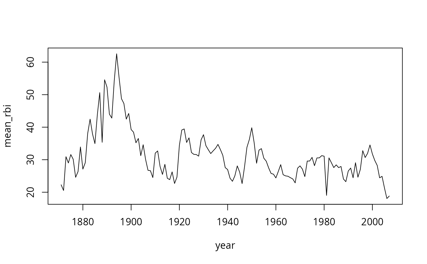
# Calculate mean runs batted in for each year
rbi <- ddply(baseball, .(year), summarise,
  mean_rbi = mean(rbi, na.rm = TRUE))
# Plot a line chart of the result
plot(mean_rbi ~ year, type = "l", data = rbi)


# make new variable career_year based on the
# start year for each player (id)
base2 <- ddply(baseball, .(id), mutate,
 career_year = year - min(year) + 1
)