Extended log-F model with fixed scale
elf.RdThe elf family implements the Extended log-F density of Fasiolo et al. (2017) and it is supposed
to work in conjuction with the extended GAM methods of Wood et al. (2017), implemented by
mgcv. It differs from the elflss family, because here the scale of the density (sigma, aka the learning rate) is a single scalar,
while in elflss it can depend on the covariates. At the moment the family is mainly intended for internal use,
use the qgam function to fit quantile GAMs based on ELF.
Arguments
- theta
a scalar representing the log-scale log(sigma).
- link
the link function between the linear predictor and the quantile location.
- qu
parameter in (0, 1) representing the chosen quantile. For instance, to fit the median choose
qu=0.5.- co
positive constant used to determine parameter lambda of the ELF density (lambda = co / sigma). Can be vector valued.
References
Fasiolo, M., Wood, S.N., Zaffran, M., Nedellec, R. and Goude, Y., 2020. Fast calibrated additive quantile regression. Journal of the American Statistical Association (to appear). doi:10.1080/01621459.2020.1725521 .
Wood, Simon N., Pya, N. and Safken, B. (2017). Smoothing parameter and model selection for general smooth models. Journal of the American Statistical Association.
Author
Matteo Fasiolo <[email protected]> and Simon N. Wood.
Examples
library(qgam)
set.seed(2)
dat <- gamSim(1,n=400,dist="normal",scale=2)
#> Gu & Wahba 4 term additive model
# Fit median using elf directly: FAST BUT NOT RECOMMENDED
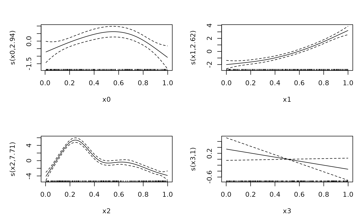
fit <- gam(y~s(x0)+s(x1)+s(x2)+s(x3),
family = elf(co = 0.1, qu = 0.5), data = dat)
plot(fit, scale = FALSE, pages = 1)
 # Using qgam: RECOMMENDED
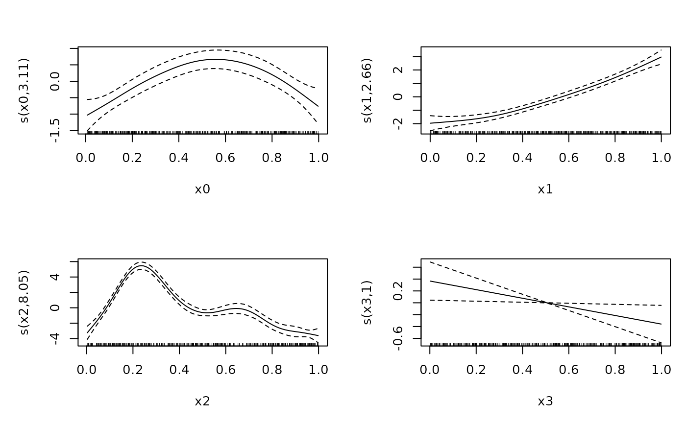
fit <- qgam(y~s(x0)+s(x1)+s(x2)+s(x3), data=dat, qu = 0.8)
#> Estimating learning rate. Each dot corresponds to a loss evaluation.
#> qu = 0.8.........done
plot(fit, scale = FALSE, pages = 1)
# Using qgam: RECOMMENDED
fit <- qgam(y~s(x0)+s(x1)+s(x2)+s(x3), data=dat, qu = 0.8)
#> Estimating learning rate. Each dot corresponds to a loss evaluation.
#> qu = 0.8.........done
plot(fit, scale = FALSE, pages = 1)