Fit a smooth additive quantile regression model

This function fits a smooth additive regression model for a single quantile.

Usage

qgam(
  form,
  data,
  qu,
  discrete = FALSE,
  lsig = NULL,
  err = NULL,
  multicore = !is.null(cluster),
  cluster = NULL,
  ncores = detectCores() - 1,
  paropts = list(),
  control = list(),
  argGam = NULL
)

Arguments

form: A GAM formula, or a list of formulae. See ?mgcv::gam details.
data: A data frame or list containing the model response variable and covariates required by the formula. By default the variables are taken from environment(formula): typically the environment from which gam is called.
qu: The quantile of interest. Should be in (0, 1).
discrete: If TRUE then covariate discretisation is used for faster model fitting. See mgcv::bam for details.
lsig: The value of the log learning rate used to create the Gibbs posterior. By defauls lsig=NULL and this parameter is estimated by posterior calibration described in Fasiolo et al. (2017). Obviously, the function is much faster if the user provides a value.
err: An upper bound on the error of the estimated quantile curve. Should be in (0, 1). Since qgam v1.3 it is selected automatically, using the methods of Fasiolo et al. (2017). The old default was err=0.05.
multicore: If TRUE the calibration will happen in parallel.
cluster: An object of class c("SOCKcluster", "cluster"). This allowes the user to pass her own cluster, which will be used if multicore == TRUE. The user has to remember to stop the cluster.
ncores: Number of cores used. Relevant if multicore == TRUE.
paropts: a list of additional options passed into the foreach function when parallel computation is enabled. This is important if (for example) your code relies on external data or packages: use the .export and .packages arguments to supply them so that all cluster nodes have the correct environment set up for computing.
control: A list of control parameters. The only one relevant here is link, which is the link function used (see ?elf and ?elflss for defaults). All other control parameters are used by tuneLearnFast. See ?tuneLearnFast for details.
argGam: A list of parameters to be passed to mgcv::gam. This list can potentially include all the arguments listed in ?gam, with the exception of formula, family and data.

Value

A gamObject. See ?gamObject.

References

Fasiolo, M., Wood, S.N., Zaffran, M., Nedellec, R. and Goude, Y., 2020. Fast calibrated additive quantile regression. Journal of the American Statistical Association (to appear). doi:10.1080/01621459.2020.1725521 .

Fasiolo, M., Wood, S.N., Zaffran, M., Nedellec, R. and Goude, Y., 2021. qgam: Bayesian Nonparametric Quantile Regression Modeling in R. Journal of Statistical Software, 100(9), 1-31, doi:10.18637/jss.v100.i09 .

Author

Matteo Fasiolo <[email protected]>.

Examples

#####
# Univariate "car" example
####
library(qgam); library(MASS)

# Fit for quantile 0.5 using the best sigma
set.seed(6436)
fit <- qgam(accel~s(times, k=20, bs="ad"), data = mcycle, qu = 0.5)
#> Estimating learning rate. Each dot corresponds to a loss evaluation. 
#> qu = 0.5........done 

# Plot the fit
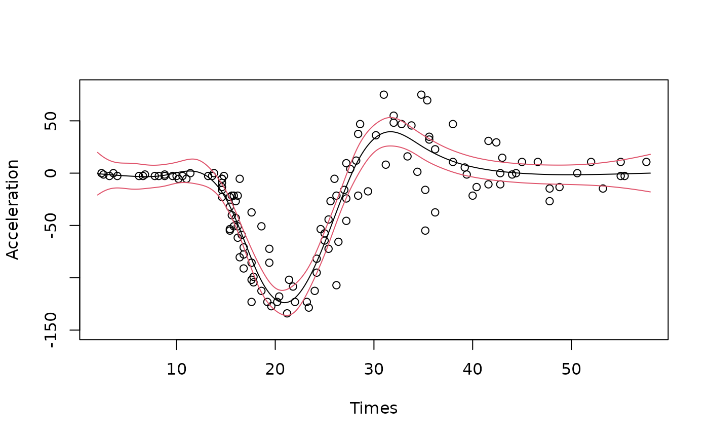
xSeq <- data.frame(cbind("accel" = rep(0, 1e3), "times" = seq(2, 58, length.out = 1e3)))
pred <- predict(fit, newdata = xSeq, se=TRUE)
plot(mcycle$times, mcycle$accel, xlab = "Times", ylab = "Acceleration", ylim = c(-150, 80))
lines(xSeq$times, pred$fit, lwd = 1)
lines(xSeq$times, pred$fit + 2*pred$se.fit, lwd = 1, col = 2)
lines(xSeq$times, pred$fit - 2*pred$se.fit, lwd = 1, col = 2)   


if (FALSE) { # \dontrun{
# You can get a better fit by letting the learning rate change with "accel"
# For instance
fit <- qgam(list(accel ~ s(times, k=20, bs="ad"), ~ s(times)),
           data = mcycle, qu = 0.8)

pred <- predict(fit, newdata = xSeq, se=TRUE)
plot(mcycle$times, mcycle$accel, xlab = "Times", ylab = "Acceleration", ylim = c(-150, 80))
lines(xSeq$times, pred$fit, lwd = 1)
lines(xSeq$times, pred$fit + 2*pred$se.fit, lwd = 1, col = 2)
lines(xSeq$times, pred$fit - 2*pred$se.fit, lwd = 1, col = 2)  
} # }

#####
# Multivariate Gaussian example
####
library(qgam)
set.seed(2)
dat <- gamSim(1,n=400,dist="normal",scale=2)
#> Gu & Wahba 4 term additive model

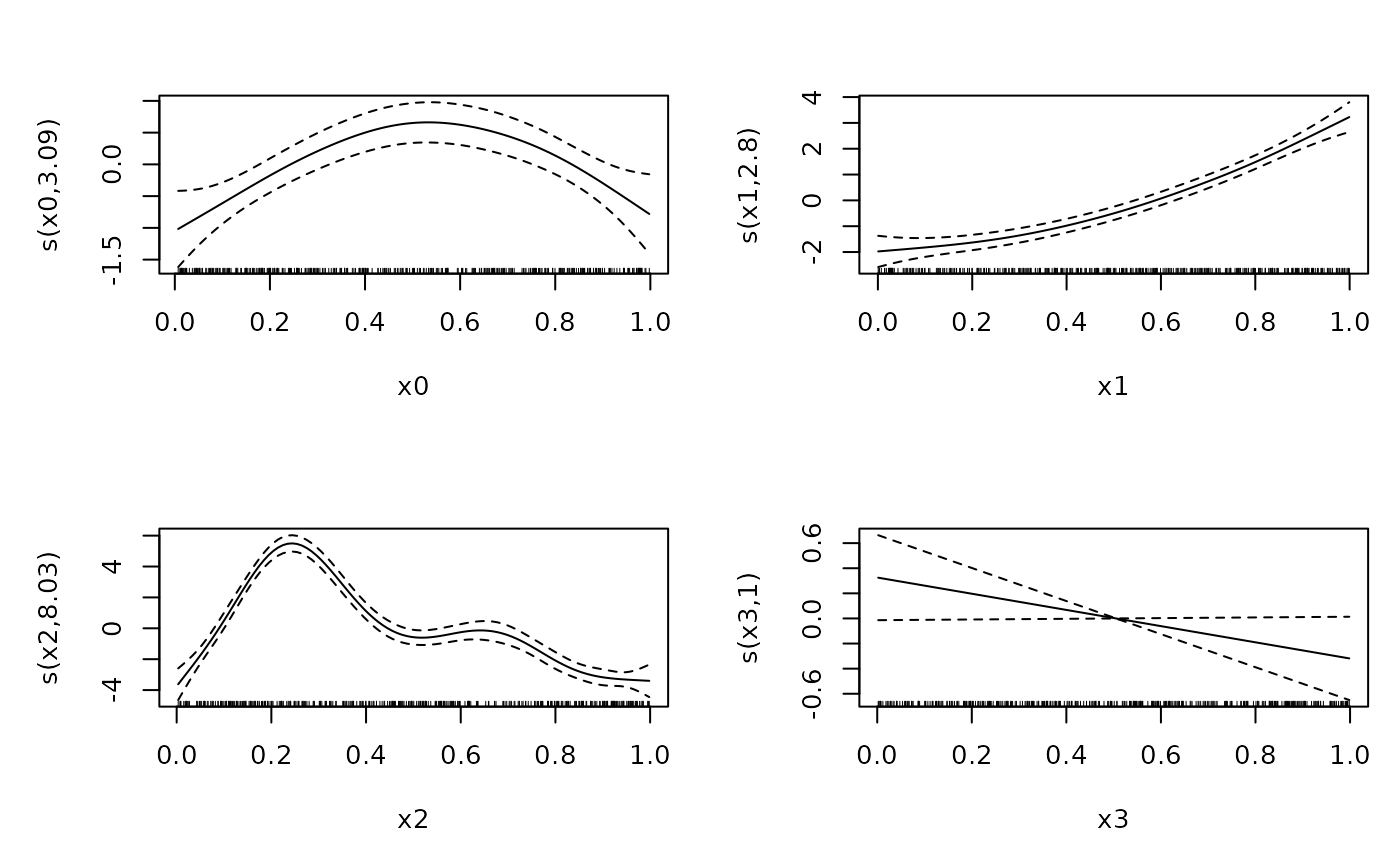
fit <- qgam(y~s(x0)+s(x1)+s(x2)+s(x3), data=dat, qu = 0.5)
#> Estimating learning rate. Each dot corresponds to a loss evaluation. 
#> qu = 0.5.......done 
plot(fit, scale = FALSE, pages = 1)      


######
# Heteroscedastic example
######
if (FALSE) { # \dontrun{
set.seed(651)
n <- 2000
x <- seq(-4, 3, length.out = n)
X <- cbind(1, x, x^2)
beta <- c(0, 1, 1)
sigma =  1.2 + sin(2*x)
f <- drop(X %*% beta)
dat <- f + rnorm(n, 0, sigma)
dataf <- data.frame(cbind(dat, x))
names(dataf) <- c("y", "x")

fit <- qgam(list(y~s(x, k = 30, bs = "cr"), ~ s(x, k = 30, bs = "cr")), 
            data = dataf, qu = 0.95)

plot(x, dat, col = "grey", ylab = "y")
tmp <- predict(fit, se = TRUE)
lines(x, tmp$fit)
lines(x, tmp$fit + 2 * tmp$se.fit, col = 2)
lines(x, tmp$fit - 2 * tmp$se.fit, col = 2)
} # }