A note about the speed of the functional form for rxode2
The functional form has the benefit that it is what is supported by nlmixr2 and therefore there is only one interface between solving and estimating, and it takes some computation time to get to the underlying “classic” simulation code.
These models are in the form of:
library(rxode2)
#> rxode2 4.0.3 using 2 threads (see ?getRxThreads)
#>   no cache: create with `rxCreateCache()`

mod1 <- function() {
  ini({
    KA   <- 0.3
    CL   <- 7
    V2   <- 40
    Q    <- 10
    V3   <- 300
    Kin  <- 0.2
    Kout <- 0.2
    EC50 <- 8
  })
  model({
    C2 = centr/V2
    C3 = peri/V3
    d/dt(depot) = -KA*depot
    d/dt(centr) = KA*depot - CL*C2 - Q*C2 + Q*C3
    d/dt(peri) = Q*C2 - Q*C3
    d/dt(eff) = Kin - Kout*(1-C2/(EC50+C2))*eff
    eff(0) = 1
  })
}
Or you can also specify the end-points for simulation/estimation just like nlmixr2:
mod2f <- function() {
  ini({
    TKA   <- 0.3
    TCL   <- 7
    TV2   <- 40
    TQ    <- 10
    TV3   <- 300
    TKin  <- 0.2
    TKout <- 0.2
    TEC50 <- 8
    eta.cl + eta.v ~ c(0.09,
                       0.08, 0.25)
    c2.prop.sd <- 0.1
    eff.add.sd <- 0.1
  })
  model({
    KA <- TKA
    CL <- TCL*exp(eta.cl)
    V2  <- TV2*exp(eta.v)
    Q   <- TQ
    V3  <- TV3
    Kin  <- TKin
    Kout <- TKout
    EC50 <- TEC50
    C2 = centr/V2
    C3 = peri/V3
    d/dt(depot) = -KA*depot
    d/dt(centr) = KA*depot - CL*C2 - Q*C2 + Q*C3
    d/dt(peri) = Q*C2 - Q*C3
    d/dt(eff) = Kin - Kout*(1-C2/(EC50+C2))*eff
    eff(0) = 1
    C2 ~ prop(c2.prop.sd)
    eff ~ add(eff.add.sd)
  })
}
For every solve, there is a compile (or a cached compile) of the underlying model. If you wish to speed this process up you can use the two underlying rxode2 classic models. This takes two steps:
Parsing/evaluating the model
Creating the simulation model
The first step can be done by rxode2(mod1) or mod1() (or for the second model too).
mod1 <- mod1()
mod2f <- rxode2(mod2f)
#> ℹ parameter labels from comments are typically ignored in non-interactive mode
#> ℹ Need to run with the source intact to parse comments
The second step is to create the underlying “classic” rxode2 model, which can be done with two different methods:$simulationModel and $simulationIniModel. The $simulationModel will provide the simulation code without the initial conditions pre-pended, the $simulationIniModel will pre-pend the values. When the endpoints are specified, the simulation code for each endpoint is also output. You can see the differences below:
summary(mod1$simulationModel)
#> rxode2 4.0.3 model named rx_3b133ba4b34510355037c48c6eb84b01 model (✔ ready).
#> DLL: /tmp/Rtmp2nePyq/rxode2/rx_3b133ba4b34510355037c48c6eb84b01__.rxd/rx_3b133ba4b34510355037c48c6eb84b01_.so
#> NULL
#>
#> Calculated Variables:
#> [1] "C2" "C3"
#> ── rxode2 Model Syntax ──
#> rxode2({
#>     param(KA, CL, V2, Q, V3, Kin, Kout, EC50)
#>     C2 = centr/V2
#>     C3 = peri/V3
#>     d/dt(depot) = -KA * depot
#>     d/dt(centr) = KA * depot - CL * C2 - Q * C2 + Q * C3
#>     d/dt(peri) = Q * C2 - Q * C3
#>     d/dt(eff) = Kin - Kout * (1 - C2/(EC50 + C2)) * eff
#>     eff(0) = 1
#> })
summary(mod1$simulationIniModel)
#> using C compiler: ‘gcc (Ubuntu 11.4.0-1ubuntu1~22.04) 11.4.0’
#> rxode2 4.0.3 model named rx_830386fbebba2e612b55aebd728b4ec1 model (✔ ready).
#> DLL: /tmp/Rtmp2nePyq/rxode2/rx_830386fbebba2e612b55aebd728b4ec1__.rxd/rx_830386fbebba2e612b55aebd728b4ec1_.so
#> NULL
#>
#> Calculated Variables:
#> [1] "C2" "C3"
#> ── rxode2 Model Syntax ──
#> rxode2({
#>     param(KA, CL, V2, Q, V3, Kin, Kout, EC50)
#>     KA = 0.3
#>     CL = 7
#>     V2 = 40
#>     Q = 10
#>     V3 = 300
#>     Kin = 0.2
#>     Kout = 0.2
#>     EC50 = 8
#>     C2 = centr/V2
#>     C3 = peri/V3
#>     d/dt(depot) = -KA * depot
#>     d/dt(centr) = KA * depot - CL * C2 - Q * C2 + Q * C3
#>     d/dt(peri) = Q * C2 - Q * C3
#>     d/dt(eff) = Kin - Kout * (1 - C2/(EC50 + C2)) * eff
#>     eff(0) = 1
#> })
summary(mod2f$simulationModel)
#> using C compiler: ‘gcc (Ubuntu 11.4.0-1ubuntu1~22.04) 11.4.0’
#> rxode2 4.0.3 model named rx_22c06be5105cba0dbc343ea7644b0a15 model (✔ ready).
#> DLL: /tmp/Rtmp2nePyq/rxode2/rx_22c06be5105cba0dbc343ea7644b0a15__.rxd/rx_22c06be5105cba0dbc343ea7644b0a15_.so
#> NULL
#>
#> Calculated Variables:
#>  [1] "KA"       "CL"       "V2"       "Q"        "V3"       "Kin"
#>  [7] "Kout"     "EC50"     "C2"       "C3"       "ipredSim" "sim"
#> ── rxode2 Model Syntax ──
#> rxode2({
#>     param(TKA, TCL, TV2, TQ, TV3, TKin, TKout, TEC50, c2.prop.sd,
#>         eff.add.sd, eta.cl, eta.v)
#>     KA = TKA
#>     CL = TCL * exp(eta.cl)
#>     V2 = TV2 * exp(eta.v)
#>     Q = TQ
#>     V3 = TV3
#>     Kin = TKin
#>     Kout = TKout
#>     EC50 = TEC50
#>     C2 = centr/V2
#>     C3 = peri/V3
#>     d/dt(depot) = -KA * depot
#>     d/dt(centr) = KA * depot - CL * C2 - Q * C2 + Q * C3
#>     d/dt(peri) = Q * C2 - Q * C3
#>     d/dt(eff) = Kin - Kout * (1 - C2/(EC50 + C2)) * eff
#>     eff(0) = 1
#>     if (CMT == 5) {
#>         rx_yj_ ~ 2
#>         rx_lambda_ ~ 1
#>         rx_low_ ~ 0
#>         rx_hi_ ~ 1
#>         rx_pred_f_ ~ C2
#>         rx_pred_ ~ rx_pred_f_
#>         rx_r_ ~ (rx_pred_f_ * c2.prop.sd)^2
#>         ipredSim = rxTBSi(rx_pred_, rx_lambda_, rx_yj_, rx_low_,
#>             rx_hi_)
#>         sim = rxTBSi(rx_pred_ + sqrt(rx_r_) * rxerr.C2, rx_lambda_,
#>             rx_yj_, rx_low_, rx_hi_)
#>     }
#>     if (CMT == 4) {
#>         rx_yj_ ~ 2
#>         rx_lambda_ ~ 1
#>         rx_low_ ~ 0
#>         rx_hi_ ~ 1
#>         rx_pred_f_ ~ eff
#>         rx_pred_ ~ rx_pred_f_
#>         rx_r_ ~ (eff.add.sd)^2
#>         ipredSim = rxTBSi(rx_pred_, rx_lambda_, rx_yj_, rx_low_,
#>             rx_hi_)
#>         sim = rxTBSi(rx_pred_ + sqrt(rx_r_) * rxerr.eff, rx_lambda_,
#>             rx_yj_, rx_low_, rx_hi_)
#>     }
#>     cmt(C2)
#>     dvid(5, 4)
#> })
summary(mod2f$simulationIniModel)
#> using C compiler: ‘gcc (Ubuntu 11.4.0-1ubuntu1~22.04) 11.4.0’
#> rxode2 4.0.3 model named rx_0fe785b5a9fbeb984fc99d0f5a550cc5 model (✔ ready).
#> DLL: /tmp/Rtmp2nePyq/rxode2/rx_0fe785b5a9fbeb984fc99d0f5a550cc5__.rxd/rx_0fe785b5a9fbeb984fc99d0f5a550cc5_.so
#> NULL
#>
#> Calculated Variables:
#>  [1] "KA"       "CL"       "V2"       "Q"        "V3"       "Kin"
#>  [7] "Kout"     "EC50"     "C2"       "C3"       "ipredSim" "sim"
#> ── rxode2 Model Syntax ──
#> rxode2({
#>     param(TKA, TCL, TV2, TQ, TV3, TKin, TKout, TEC50, c2.prop.sd,
#>         eff.add.sd, eta.cl, eta.v)
#>     rxerr.C2 = 1
#>     rxerr.eff = 1
#>     TKA = 0.3
#>     TCL = 7
#>     TV2 = 40
#>     TQ = 10
#>     TV3 = 300
#>     TKin = 0.2
#>     TKout = 0.2
#>     TEC50 = 8
#>     c2.prop.sd = 0.1
#>     eff.add.sd = 0.1
#>     eta.cl = 0
#>     eta.v = 0
#>     KA = TKA
#>     CL = TCL * exp(eta.cl)
#>     V2 = TV2 * exp(eta.v)
#>     Q = TQ
#>     V3 = TV3
#>     Kin = TKin
#>     Kout = TKout
#>     EC50 = TEC50
#>     C2 = centr/V2
#>     C3 = peri/V3
#>     d/dt(depot) = -KA * depot
#>     d/dt(centr) = KA * depot - CL * C2 - Q * C2 + Q * C3
#>     d/dt(peri) = Q * C2 - Q * C3
#>     d/dt(eff) = Kin - Kout * (1 - C2/(EC50 + C2)) * eff
#>     eff(0) = 1
#>     if (CMT == 5) {
#>         rx_yj_ ~ 2
#>         rx_lambda_ ~ 1
#>         rx_low_ ~ 0
#>         rx_hi_ ~ 1
#>         rx_pred_f_ ~ C2
#>         rx_pred_ ~ rx_pred_f_
#>         rx_r_ ~ (rx_pred_f_ * c2.prop.sd)^2
#>         ipredSim = rxTBSi(rx_pred_, rx_lambda_, rx_yj_, rx_low_,
#>             rx_hi_)
#>         sim = rxTBSi(rx_pred_ + sqrt(rx_r_) * rxerr.C2, rx_lambda_,
#>             rx_yj_, rx_low_, rx_hi_)
#>     }
#>     if (CMT == 4) {
#>         rx_yj_ ~ 2
#>         rx_lambda_ ~ 1
#>         rx_low_ ~ 0
#>         rx_hi_ ~ 1
#>         rx_pred_f_ ~ eff
#>         rx_pred_ ~ rx_pred_f_
#>         rx_r_ ~ (eff.add.sd)^2
#>         ipredSim = rxTBSi(rx_pred_, rx_lambda_, rx_yj_, rx_low_,
#>             rx_hi_)
#>         sim = rxTBSi(rx_pred_ + sqrt(rx_r_) * rxerr.eff, rx_lambda_,
#>             rx_yj_, rx_low_, rx_hi_)
#>     }
#>     cmt(C2)
#>     dvid(5, 4)
#> })
If you wish to speed up multiple simualtions from the rxode2 functions, you need to pre-calculate care of the steps above:
mod1 <- mod1$simulationModel

mod2 <- mod2f$simulationModel
These functions then can act like a normal ui model to be solved. You can convert them back to a UI as.rxUi() or a function as.function() as needed.
To increase speed for multiple simulations from the same model you should use the lower level simulation model (ie $simulationModel or $simulationIniModel depending on what you need)
Increasing rxode2 speed by multi-subject parallel solving
Using the classic rxode2 model specification (which we can convert from a functional/ui model style) we will continue the discussion on rxode2 speed enhancements.
rxode2 originally developed as an ODE solver that allowed an ODE solve for a single subject. This flexibility is still supported.
The original code from the rxode2 tutorial is below:
library(rxode2)

library(microbenchmark)
library(ggplot2)

mod1 <- rxode2({
    C2 = centr/V2
    C3 = peri/V3
    d/dt(depot) = -KA*depot
    d/dt(centr) = KA*depot - CL*C2 - Q*C2 + Q*C3
    d/dt(peri) = Q*C2 - Q*C3
    d/dt(eff) = Kin - Kout*(1-C2/(EC50+C2))*eff
    eff(0) = 1
})
#> using C compiler: ‘gcc (Ubuntu 11.4.0-1ubuntu1~22.04) 11.4.0’

## Create an event table

ev <- et() %>%
    et(amt=10000, addl=9,ii=12) %>%
    et(time=120, amt=20000, addl=4, ii=24) %>%
    et(0:240) ## Add Sampling

nsub <- 100 # 100 sub-problems
sigma <- matrix(c(0.09,0.08,0.08,0.25),2,2) # IIV covariance matrix
mv <- rxRmvn(n=nsub, rep(0,2), sigma) # Sample from covariance matrix
CL <- 7*exp(mv[,1])
V2 <- 40*exp(mv[,2])
params.all <- cbind(KA=0.3, CL=CL, V2=V2, Q=10, V3=300,
                    Kin=0.2, Kout=0.2, EC50=8)
For Loop
The slowest way to code this is to use a for loop. In this example we will enclose it in a function to compare timing.
Running with apply
In general for R, the apply types of functions perform better than a for loop, so the tutorial also suggests this speed enhancement
runSapply <- function(){
    res <- apply(params.all, 1, function(theta)
        mod1$run(theta, ev)[, "eff"])
}
Run using a single-threaded solve
You can also have rxode2 solve all the subject simultaneously without collecting the results in R, using a single threaded solve.
The data output is slightly different here, but still gives the same information:
Run a 2 threaded solve
rxode2 supports multi-threaded solves, so another option is to have 2 threads (called cores in the solve options, you can see the options in rxControl() or rxSolve()).
Compare the times between all the methods
Now the moment of truth, the timings:
bench <- microbenchmark(runFor(), runSapply(), runSingleThread(),run2Thread())
print(bench)
#> Unit: milliseconds
#>               expr       min        lq      mean    median        uq       max
#>           runFor() 395.21576 423.29853 468.85968 454.27117 478.09516 690.68592
#>        runSapply() 393.16993 415.42880 472.45963 461.65203 488.72941 739.52423
#>  runSingleThread()  26.53470  27.37301  30.63664  28.07569  30.71933  46.34973
#>       run2Thread()  17.79166  20.62662  26.15072  24.46771  27.44174 187.70665
#>  neval
#>    100
#>    100
#>    100
#>    100
autoplot(bench)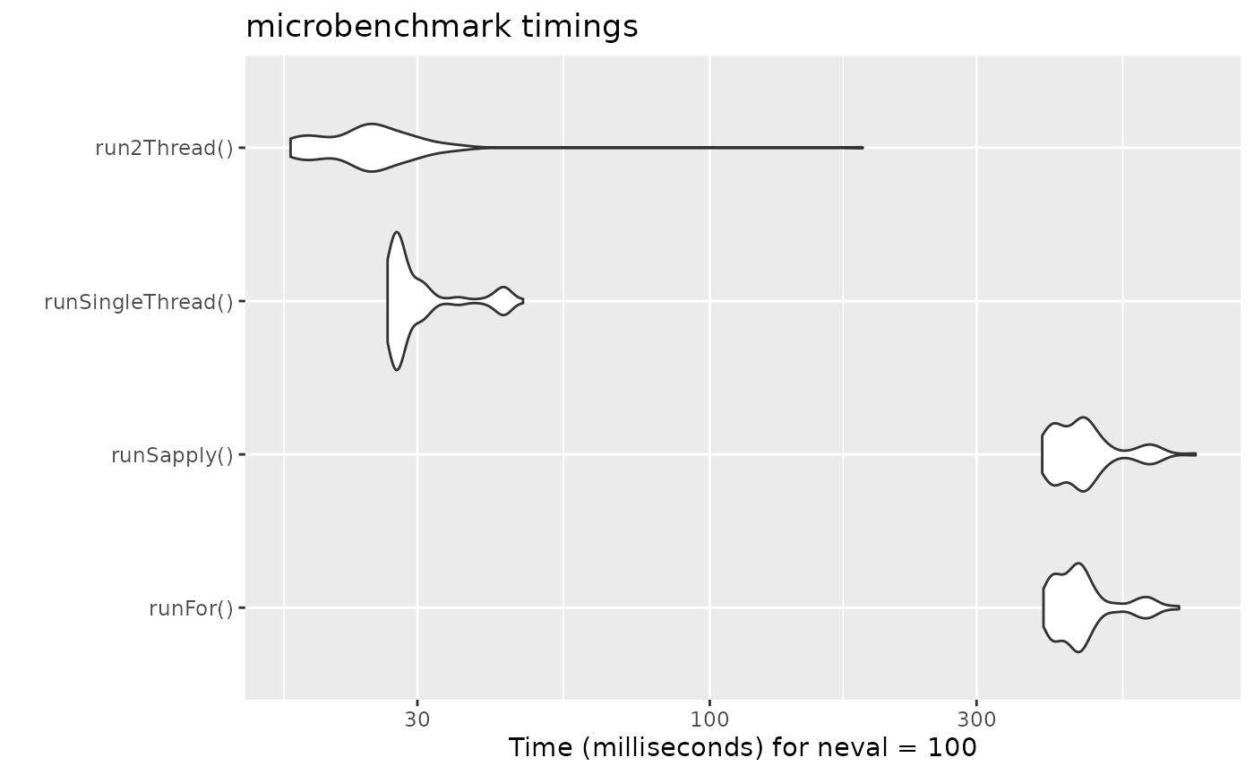
It is clear that the largest jump in performance when using the solve method and providing all the parameters to rxode2 to solve without looping over each subject with either a for or a sapply. The number of cores/threads applied to the solve also plays a role in the solving.
We can explore the number of threads further with the following code:
runThread <- function(n){
    solve(mod1, params.all, ev, cores=n)[,c("sim.id", "time", "eff")]
}

bench <- eval(parse(text=sprintf("microbenchmark(%s)",
                                     paste(paste0("runThread(", seq(1, 2 * rxCores()),")"),
                                           collapse=","))))
print(bench)
#> Unit: milliseconds
#>          expr      min       lq     mean   median       uq      max neval
#>  runThread(1) 26.76294 27.52830 32.60908 28.72995 36.06078 53.26970   100
#>  runThread(2) 23.54294 24.81824 26.90235 25.60302 28.39930 38.32454   100
#>  runThread(3) 19.79845 20.68153 24.66119 22.17414 26.90559 48.60789   100
#>  runThread(4) 23.85542 26.45917 29.29665 28.56387 30.30504 54.19030   100
autoplot(bench)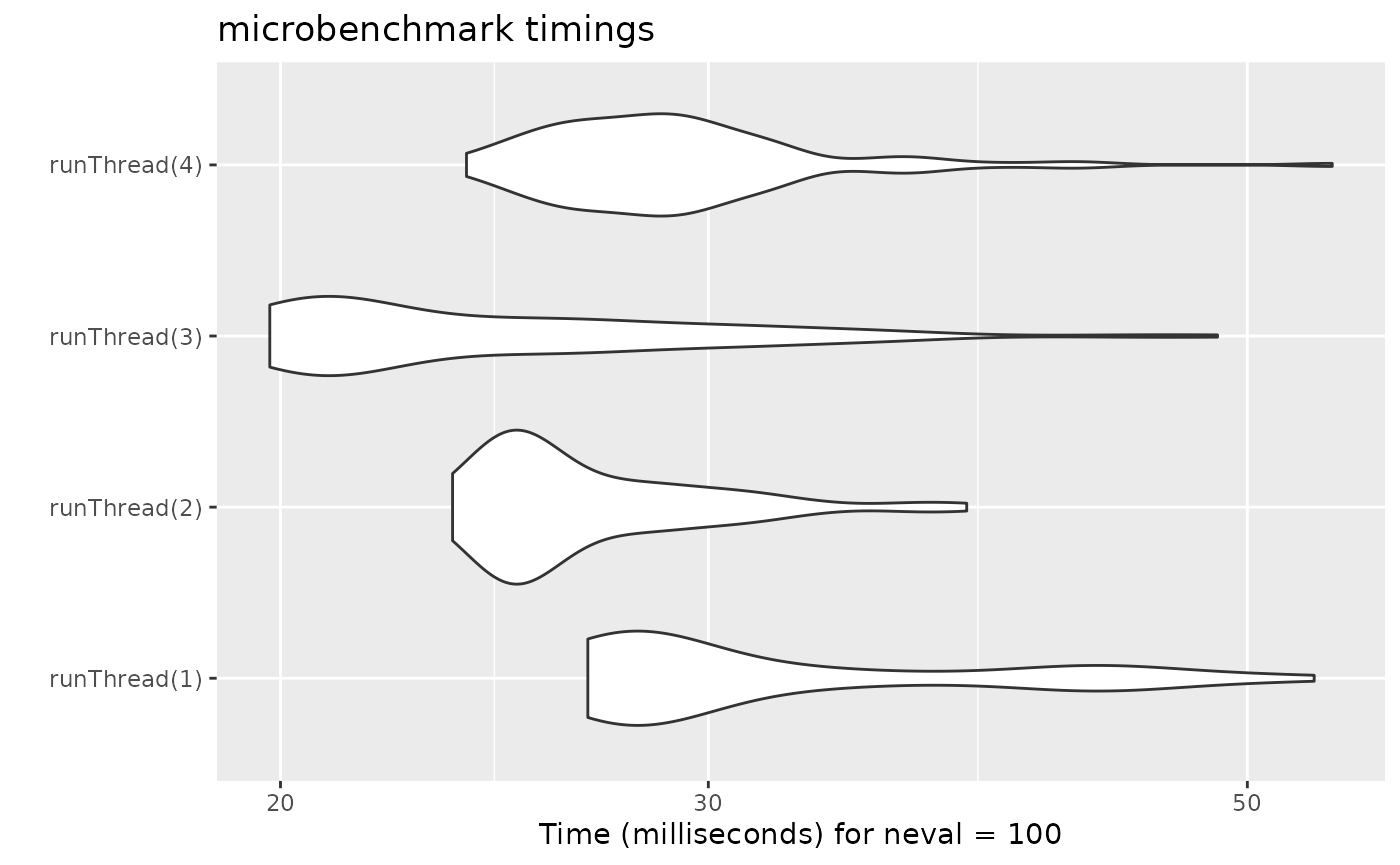
There can be a suite spot in speed vs number or cores. The system type (mac, linux, windows and/or processor), complexity of the ODE solving and the number of subjects may affect this arbitrary number of threads. 4 threads is a good number to use without any prior knowledge because most systems these days have at least 4 threads (or 2 processors with 4 threads).
Increasing speed with compiler options
One of the way that allows faster ODE solving is to make some approximations that make some math operators like exp() faster but not technically accurate enough to follow the IEEE standard for the math functions values (there are other implications that I will not cover here).
While these are optimizations are opt-in for Julia since they compile everything each session, CRAN has a more conservative approach since individuals do not compile each R function before running it.
Still, rxode2 models can be compiled with this option without disturbing CRAN policies. The key is to set an option. Here is an example:
# Using the first example subset to PK
mod2f <- function() {
  ini({
    TKA   <- 0.3
    TCL   <- 7
    TV2   <- 40
    TQ    <- 10
    TV3   <- 300
    TKin  <- 0.2
    TKout <- 0.2
    TEC50 <- 8
    eta.cl + eta.v ~ c(0.09,
                       0.08, 0.25)
    c2.prop.sd <- 0.1
  })
  model({
    KA <- TKA
    CL <- TCL*exp(eta.cl)
    V2  <- TV2*exp(eta.v)
    Q   <- TQ
    V3  <- TV3
    Kin  <- TKin
    Kout <- TKout
    EC50 <- TEC50
    C2 = centr/V2
    C3 = peri/V3
    d/dt(depot) = -KA*depot
    d/dt(centr) = KA*depot - CL*C2 - Q*C2 + Q*C3
    d/dt(peri) = Q*C2 - Q*C3
    C2 ~ prop(c2.prop.sd)
  })
}

mod2f <- mod2f()

mod2s <- mod2f$simulationIniModel
#> using C compiler: ‘gcc (Ubuntu 11.4.0-1ubuntu1~22.04) 11.4.0’

ev  <- et(amountUnits="mg", timeUnits="hours") %>%
  et(amt=10000, addl=9,ii=12,cmt="depot") %>%
  et(time=120, amt=2000, addl=4, ii=14, cmt="depot") %>%
  et(0:240) # Add sampling

bench1 <- microbenchmark(standardCompile=rxSolve(mod2s, ev, nSub=1000))

# Now clear the cache of models so we can change the compile options for the same model
rxClean()

# Use withr to preserve the options
withr::with_options(list(rxode2.compile.O="fast"), {
  mod2s <- mod2f$simulationIniModel
})
#> using C compiler: ‘gcc (Ubuntu 11.4.0-1ubuntu1~22.04) 11.4.0’

bench2 <- microbenchmark(fastCompile=rxSolve(mod2s, ev, nSub=1000))

bench <- rbind(bench1, bench2)

print(bench)
#> Unit: milliseconds
#>             expr      min       lq     mean   median       uq      max neval
#>  standardCompile 379.2977 404.2832 491.5483 525.6018 572.8156 620.8875   100
#>      fastCompile 382.6057 406.9777 495.2016 502.3768 574.3354 716.3196   100

autoplot(bench)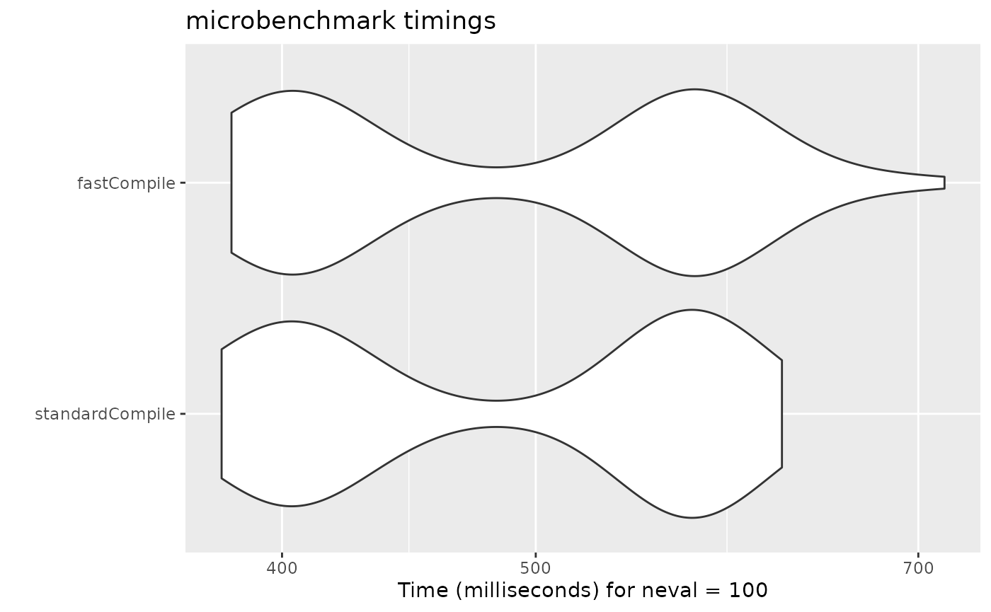
Note compiler settings can be tricky and if you setup your system wide Makevars it may interact with this setting. For example if you use ccache the compile may not be produced with the same options since it was cached with the other options.
For example, on the github runner (which generates this page), there is no advantage to the "fast" compile. However, on my development laptop there is some minimal speed increase. You should probably check before using this yourself.
This is disabled by default since there is only minimum increase in speed.
A real life example
cBefore some of the parallel solving was implemented, the fastest way to run rxode2 was with lapply. This is how Rik Schoemaker created the data-set for nlmixr comparisons, but reduced to run faster automatic building of the pkgdown website.
library(rxode2)
library(data.table)
#Define the rxode2 model
  ode1 <- "
  d/dt(abs)    = -KA*abs;
  d/dt(centr)  =  KA*abs-(CL/V)*centr;
  C2=centr/V;
  "

#Create the rxode2 simulation object
mod1 <- rxode2(model = ode1)
#> using C compiler: ‘gcc (Ubuntu 11.4.0-1ubuntu1~22.04) 11.4.0’

#Population parameter values on log-scale
  paramsl <- c(CL = log(4),
               V = log(70),
               KA = log(1))
#make 10,000 subjects to sample from:
  nsubg <- 300 # subjects per dose
  doses <- c(10, 30, 60, 120)
  nsub <- nsubg * length(doses)
#IIV of 30% for each parameter
  omega <- diag(c(0.09, 0.09, 0.09))# IIV covariance matrix
  sigma <- 0.2
#Sample from the multivariate normal
  set.seed(98176247)
  rxSetSeed(98176247)
  library(MASS)
  mv <-
    mvrnorm(nsub, rep(0, dim(omega)[1]), omega) # Sample from covariance matrix
#Combine population parameters with IIV
  params.all <-
    data.table(
      "ID" = seq(1:nsub),
      "CL" = exp(paramsl['CL'] + mv[, 1]),
      "V" = exp(paramsl['V'] + mv[, 2]),
      "KA" = exp(paramsl['KA'] + mv[, 3])
    )
#set the doses (looping through the 4 doses)
params.all[, AMT := rep(100 * doses,nsubg)]

Startlapply <- Sys.time()

#Run the simulations using lapply for speed
  s = lapply(1:nsub, function(i) {
#selects the parameters associated with the subject to be simulated
    params <- params.all[i]
#creates an eventTable with 7 doses every 24 hours
    ev <- eventTable()
    ev$add.dosing(
      dose = params$AMT,
      nbr.doses = 1,
      dosing.to = 1,
      rate = NULL,
      start.time = 0
    )
#generates 4 random samples in a 24 hour period
    ev$add.sampling(c(0, sort(round(sample(runif(600, 0, 1440), 4) / 60, 2))))
#runs the rxode2 simulation
    x <- as.data.table(mod1$run(params, ev))
#merges the parameters and ID number to the simulation output
    x[, names(params) := params]
  })

#runs the entire sequence of 100 subjects and binds the results to the object res
  res = as.data.table(do.call("rbind", s))

Stoplapply <- Sys.time()

print(Stoplapply - Startlapply)
#> Time difference of 14.22209 secs
By applying some of the new parallel solving concepts you can simply run the same simulation both with less code and faster:
rx <- rxode2({
    CL =  log(4)
    V = log(70)
    KA = log(1)
    CL = exp(CL + eta.CL)
    V = exp(V + eta.V)
    KA = exp(KA + eta.KA)
    d/dt(abs)    = -KA*abs;
    d/dt(centr)  =  KA*abs-(CL/V)*centr;
    C2=centr/V;
})
#> using C compiler: ‘gcc (Ubuntu 11.4.0-1ubuntu1~22.04) 11.4.0’

omega <- lotri(eta.CL ~ 0.09,
               eta.V ~ 0.09,
               eta.KA ~ 0.09)

doses <- c(10, 30, 60, 120)


startParallel <- Sys.time()
ev <- do.call("rbind",
        lapply(seq_along(doses), function(i){
            et() %>%
                et(amt=doses[i]) %>% # Add single dose
                et(0) %>% # Add 0 observation
                ## Generate 4 samples in 24 hour period
                et(lapply(1:4, function(...){c(0, 24)})) %>%
                et(id=seq(1, nsubg) + (i - 1) * nsubg) %>%
                ## Convert to data frame to skip sorting the data
                ## When binding the data together
                as.data.frame
        }))
## To better compare, use the same output, that is data.table
res <- rxSolve(rx, ev, omega=omega, returnType="data.table")
endParallel <- Sys.time()
print(endParallel - startParallel)
#> Time difference of 0.124366 secs
You can see a striking time difference between the two methods; A few things to keep in mind:
rxode2use the thread-safe sitmothreefryroutines for simulation ofetavalues. Therefore the results are expected to be different (also the random samples are taken in a different order which would be different)This prior simulation was run in R 3.5, which has a different random number generator so the results in this simulation will be different from the actual nlmixr comparison when using the slower simulation.
This speed comparison used
data.table.rxode2usesdata.tableinternally (when available) try to speed up sorting, so this would be different than installations wheredata.tableis not installed. You can force rxode2 to useorder()when sorting by usingforderForceBase(TRUE). In this case there is little difference between the two, though in other examplesdata.table’s presence leads to a speed increase (and less likely it could lead to a slowdown).
Want more ways to run multi-subject simulations
The version since the tutorial has even more ways to run multi-subject simulations, including adding variability in sampling and dosing times with et() (see rxode2 events for more information), ability to supply both an omega and sigma matrix as well as adding as a thetaMat to R to simulate with uncertainty in the omega, sigma and theta matrices; see rxode2 simulation vignette.
Session Information
The session information:
sessionInfo()
#> R version 4.4.1 (2024-06-14)
#> Platform: x86_64-pc-linux-gnu
#> Running under: Ubuntu 22.04.5 LTS
#>
#> Matrix products: default
#> BLAS:   /usr/lib/x86_64-linux-gnu/openblas-pthread/libblas.so.3
#> LAPACK: /usr/lib/x86_64-linux-gnu/openblas-pthread/libopenblasp-r0.3.20.so;  LAPACK version 3.10.0
#>
#> locale:
#>  [1] LC_CTYPE=en_US.UTF-8       LC_NUMERIC=C
#>  [3] LC_TIME=en_US.UTF-8        LC_COLLATE=en_US.UTF-8
#>  [5] LC_MONETARY=en_US.UTF-8    LC_MESSAGES=en_US.UTF-8
#>  [7] LC_PAPER=en_US.UTF-8       LC_NAME=C
#>  [9] LC_ADDRESS=C               LC_TELEPHONE=C
#> [11] LC_MEASUREMENT=en_US.UTF-8 LC_IDENTIFICATION=C
#>
#> time zone: Etc/UTC
#> tzcode source: system (glibc)
#>
#> attached base packages:
#> [1] stats     graphics  grDevices utils     datasets  methods   base
#>
#> other attached packages:
#> [1] MASS_7.3-60.2        data.table_1.17.6    ggplot2_3.5.2
#> [4] microbenchmark_1.5.0 rxode2_4.0.3
#>
#> loaded via a namespace (and not attached):
#>  [1] sass_0.4.10         generics_0.1.4      lattice_0.22-6
#>  [4] digest_0.6.37       magrittr_2.0.3      evaluate_1.0.4
#>  [7] grid_4.4.1          RColorBrewer_1.1-3  fastmap_1.2.0
#> [10] lotri_1.0.0         jsonlite_2.0.0      rxode2ll_2.0.13
#> [13] backports_1.5.0     scales_1.4.0        lazyeval_0.2.2
#> [16] textshaping_1.0.1   jquerylib_0.1.4     RApiSerialize_0.1.4
#> [19] cli_3.6.5           rlang_1.1.6         symengine_0.2.10
#> [22] crayon_1.5.3        units_0.8-7         withr_3.0.2
#> [25] cachem_1.1.0        yaml_2.3.10         tools_4.4.1
#> [28] qs_0.27.3           memoise_2.0.1       checkmate_2.3.2
#> [31] dplyr_1.1.4         vctrs_0.6.5         R6_2.6.1
#> [34] lifecycle_1.0.4     fs_1.6.6            stringfish_0.16.0
#> [37] htmlwidgets_1.6.4   ragg_1.4.0          PreciseSums_0.7
#> [40] pkgconfig_2.0.3     desc_1.4.3          pkgdown_2.1.3
#> [43] RcppParallel_5.1.10 rex_1.2.1           pillar_1.10.2
#> [46] bslib_0.9.0         gtable_0.3.6        glue_1.8.0
#> [49] Rcpp_1.1.0          systemfonts_1.2.3   xfun_0.52
#> [52] tibble_3.3.0        tidyselect_1.2.1    sys_3.4.3
#> [55] knitr_1.50          farver_2.1.2        dparser_1.3.1-13
#> [58] htmltools_0.5.8.1   nlme_3.1-164        rmarkdown_2.29
#> [61] compiler_4.4.1