Quantile-based Summary Statistics for Location, Scale and Shape
qlss.RdThis function calculates quantile-based summary statistics for location, scale and shape of a distribution, unconditional or conditional.
Usage
qlss(...)
# Default S3 method
qlss(fun = "qnorm", probs = 0.1, ...)
# S3 method for class 'numeric'
qlss(x, probs = 0.1, ...)
# S3 method for class 'formula'
qlss(formula, probs = 0.1, data = sys.frame(sys.parent()), subset, weights,
  na.action, contrasts = NULL, method = "fn", type = "rq", tsf = "mcjI",
  symm = TRUE, dbounded = FALSE, lambda = NULL, conditional = FALSE, ...)
Arguments
- fun
quantile function.
- x
a numeric vector.
- formula
an object of class
formula: a symbolic description of the model to be fitted. The details of model specification are given under "Details".- probs
a vector of probabilities.
- data
an optional data frame, list or environment (or object coercible by as.data.frame to a data frame) containing the variables in the model. By default the variables are taken from the environment from which the call is made.
- subset
an optional vector specifying a subset of observations to be used in the fitting process.
- weights
an optional vector of weights to be used in the fitting process. Should be NULL or a numeric vector.
- na.action
a function which indicates what should happen when the data contain
NAs.- contrasts
an optional list. See the
contrasts.argofmodel.matrix.default.- method
the algorithm used to solve the linear program. See
rqfor further details. The Frisch-Newton interior point method is the default.- type
possible options are
rqfor linear quantile regression (default) orrqtfor transformation-based quantile regression.- tsf
transformation to be used. Possible options are
mcjIfor Proposal I transformation models (default),bcfor Box-Cox andaofor Aranda-Ordaz transformation models. Seetsrqfor further details.- symm
logical flag. If
TRUE(default) a symmetric transformation is used.- dbounded
logical flag. If
TRUEthe response is assumed to be doubly bounded on [a,b]. IfFALSEthe response is assumed to be singly bounded (ie, strictly positive).- lambda
values of transformation parameters for grid search.
- conditional
logical flag. If
TRUE, the transformation parameter is assumed to be known and this must be provided via the argumentslambdausing a vector of length3 + 2 x length(probs)(see details).- ...
other arguments for
fun,rqortsrq.
Details
This function computes a number of quantile-based summary statistics for location (median), scale (inter-quartile range and inter-quantile range), and shape (Bowley skewness and shape index) of a distribution. These statistics can be computed for unconditional and conditional distributions.
Let \(Y\) be a continuous random variable and let \(Q(p)\) be its pth quantile. The function qlss computes the median \(Q(0.5)\), the inter-quartile range \(IQR = Q(0.75) - Q(0.25)\), the inter-quantile range \(IPR(p) = Q(1-p) - Q(p)\), the Bowley skewness index \(A(p) = (Q(1-p) + Q(p) - 2Q(0.5))/IPR(p)\), and the shape index \(T(p) = IPR(p)/IQR\), for \(0 < p < 0.25\).
The default qlss function computes the summary statistics of a standard normal distribution or any other theoretical distribution via the argument fun. The latter must be a function with p as its probability argument (see for example qnorm, qt, qchisq, qgamma, etc.). When a variable x is provided, LSS measures are computed using empirical (sample) quantiles.
The argument formula specifies a quantile function for \(Y\) conditional on predictors \(X\). Linear models are fitted via standard quantile regression with type = "rq". Nonlinear models are fitted via transformation-based quantile regression with type = "rqt" (proposal II transformation models are not available.). When conditional = TRUE, lambda is a vector of transformation parameters of length 3 + 2 x np, where np = length(probs) (3 quartiles, np quantiles at level \(p\), np quantiles at level \(1 - p\)).
Value
qlss returns an object of class qlss. This is a list that contains at least three elements:
- location
summary statistic(s) for location.
- scale
summary statistic(s) for scale.
- shape
summary statistic(s) for shape.
References
Geraci M and Jones MC. Improved transformation-based quantile regression. Canadian Journal of Statistics 2015;43(1):118-132.
Gilchrist W. Statistical modelling with quantile functions. Chapman and Hall/CRC; 2000.
Examples
# Compute summary statistics of a normal distribution
qlss()
#> call:
#> qlss.default()
#>
#> Unconditional Quantile-Based Location, Scale, and Shape
#>
#> ** Location **
#> Median
#> [1] 0
#> ** Scale **
#> Inter-quartile range (IQR)
#> [1] 1.34898
#> Inter-quantile range (IPR)
#> 0.1
#> 2.563103
#> ** Shape **
#> Skewness index
#> 0.1
#> 0
#> Shape index
#> 0.1
#> 1.900031
# Compute summary statistics of a t distribution with 3 df
qlss(fun = "qt", df = 3, probs = 0.05)
#> call:
#> qlss.default(fun = "qt", probs = 0.05, df = 3)
#>
#> Unconditional Quantile-Based Location, Scale, and Shape
#>
#> ** Location **
#> Median
#> [1] 0
#> ** Scale **
#> Inter-quartile range (IQR)
#> [1] 1.529785
#> Inter-quantile range (IPR)
#> 0.05
#> 4.706727
#> ** Shape **
#> Skewness index
#> 0.05
#> -1.88704e-16
#> Shape index
#> 0.05
#> 3.076725
# Compute summary statistics for a sample using a sequence of probabilities
x <- rnorm(1000)
qlss(x, probs = c(0.1, 0.2, 0.3, 0.4))
#> call:
#> qlss.numeric(x = x, probs = c(0.1, 0.2, 0.3, 0.4))
#>
#> Unconditional Quantile-Based Location, Scale, and Shape
#>
#> ** Location **
#> Median
#> [1] -0.03489193
#> ** Scale **
#> Inter-quartile range (IQR)
#> [1] 1.282709
#> Inter-quantile range (IPR)
#> 0.1 0.2 0.3 0.4
#> 2.4557636 1.6380151 0.9847508 0.4321300
#> ** Shape **
#> Skewness index
#> 0.1 0.2 0.3 0.4
#> -0.01905402 0.00627749 0.03288934 0.11093977
#> Shape index
#> 0.1 0.2 0.3 0.4
#> 1.9145141 1.2769971 0.7677121 0.3368887
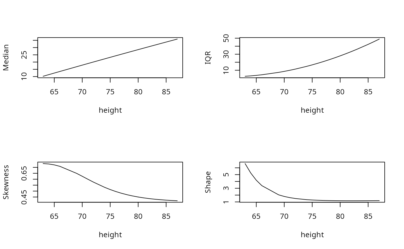
# Compute summary statistics for Volume conditional on Height
trees2 <- trees[order(trees$Height),]
fit <- qlss(Volume ~ Height, data = trees2)
#> Warning: Solution may be nonunique
plot(fit, z = trees2$Height, xlab = "height")
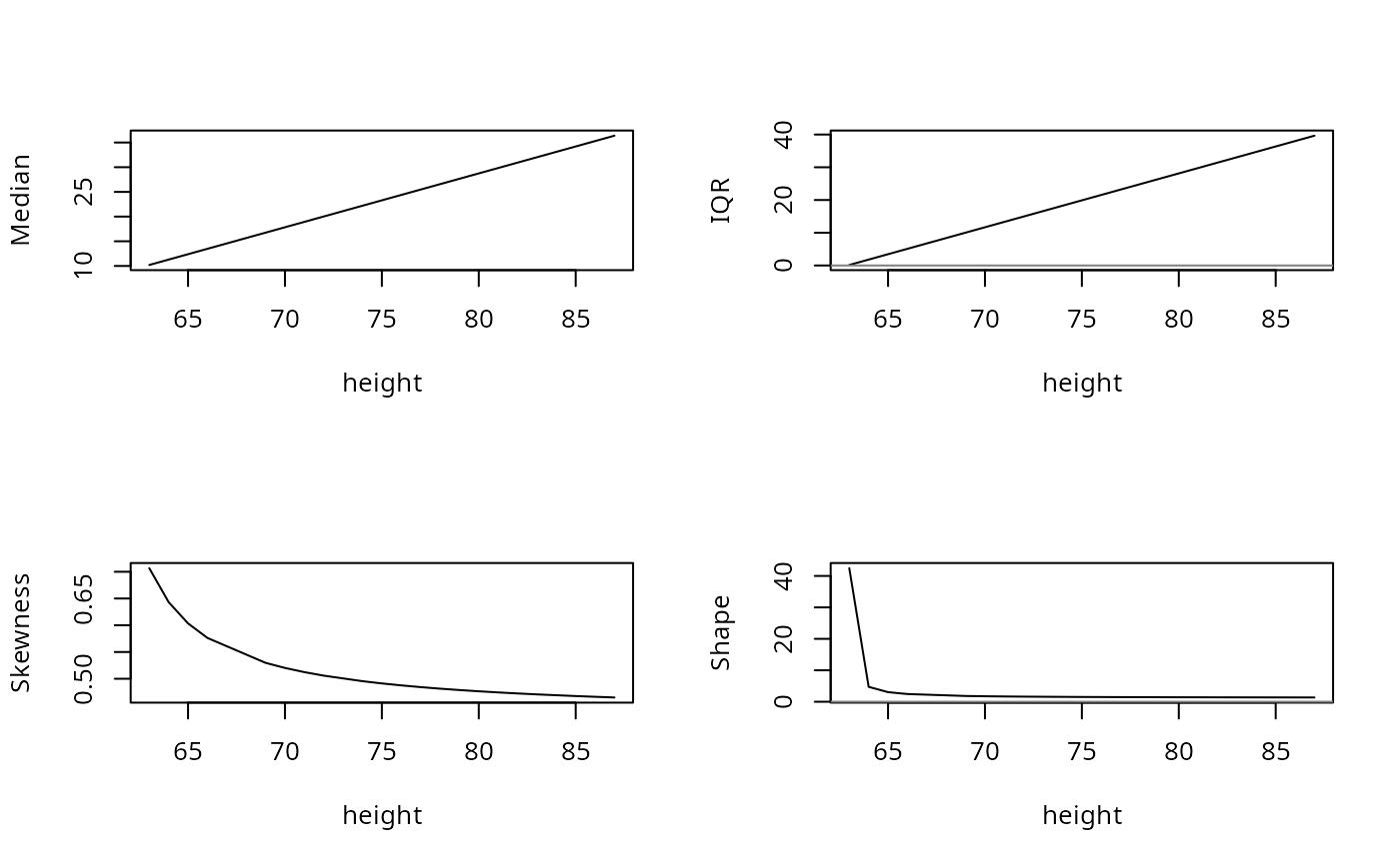 # Use a quadratic model for Height
fit <- qlss(Volume ~ poly(Height,2), data = trees2)
plot(fit, z = trees2$Height, xlab = "height")
# Use a quadratic model for Height
fit <- qlss(Volume ~ poly(Height,2), data = trees2)
plot(fit, z = trees2$Height, xlab = "height")