Illustrated quantile calculations from distributions
Usage
qdist(
  dist = "norm",
  p,
  plot = TRUE,
  verbose = FALSE,
  invisible = FALSE,
  resolution = 500L,
  digits = 3L,
  xlim,
  ylim,
  return = c("values", "plot"),
  refinements = list(),
  ...
)

xqgamma(
  p,
  shape,
  rate = 1,
  scale = 1/rate,
  lower.tail = TRUE,
  log.p = FALSE,
  ...
)

xqt(p, df, ncp, lower.tail = TRUE, log.p = FALSE, ...)

xqchisq(p, df, ncp = 0, lower.tail = TRUE, log.p = FALSE, ...)

xqf(p, df1, df2, lower.tail = TRUE, log.p = FALSE, ...)

xqbinom(p, size, prob, lower.tail = TRUE, log.p = FALSE, ...)

xqpois(p, lambda, lower.tail = TRUE, log.p = FALSE, ...)

xqgeom(p, prob, lower.tail = TRUE, log.p = FALSE, ...)

xqnbinom(p, size, prob, mu, lower.tail = TRUE, log.p = FALSE, ...)

xqbeta(p, shape1, shape2, ncp = 0, lower.tail = TRUE, log.p = FALSE, ...)
Arguments
- dist
a character description of a distribution, for example
"norm","t", or"chisq"- p
a vector of probabilities
- plot
a logical indicating whether a plot should be created
- verbose
a logical
- invisible
a logical
- resolution
number of points used for detecting discreteness and generating plots. The default value of 5000 should work well except for discrete distributions that have many distinct values, especially if these values are not evenly spaced.
- digits
the number of digits desired
- xlim
x limits. By default, these are chosen to show the central 99.8\ of the distribution.
- ylim
y limits
- return
If
"plot", return a plot. If"values", return a vector of numerical values.- refinements
A list of refinements to the plot. See
ggformula::gf_refine().- ...
additional arguments, including parameters of the distribution and additional options for the plot. To help with name collisions (eg
sizefor binomial distributions andshapefor gamma distributions), argument names beginningplot_will be renamed to removeplot_and passed only to the plot. The unprefixed version will used as a parameter for the the distribution.- shape, scale
shape and scale parameters. Must be positive,
scalestrictly.- rate
an alternative way to specify the scale.
- lower.tail
logical; if
TRUE(default), probabilities are \(P[X < x]\), otherwise, \(P[X \ge x]\) (exceptionally not cadlag here, to ensure, e.g.,pgamma(0, shape=0)remains zero).- log.p
A logical indicating whether probabilities should be returned on the log scale.
- df
degrees of freedom (\(> 0\), maybe non-integer).
df
      = Inf
is allowed.- ncp
non-centrality parameter \(\delta\); currently except for
rt(), accurate only forabs(ncp) <= 37.62. If omitted, use the central \(t\) distribution.- df1, df2
degrees of freedom.
Infis allowed.- size
number of trials (zero or more).
- prob
probability of success on each trial.
- lambda
vector of (non-negative) means.
- mu
alternative parametrization via mean: see ‘Details’.
- shape1, shape2
non-negative parameters of the Beta distribution.
Details
The most general function is qdist which can work with
any distribution for which a q-function exists. As a convenience, wrappers are
provided for several common distributions.
Examples
qdist("norm", seq(.1, .9, by = 0.10),
title = "Deciles of a normal distribution", show.legend = FALSE,
pattern = "rings")
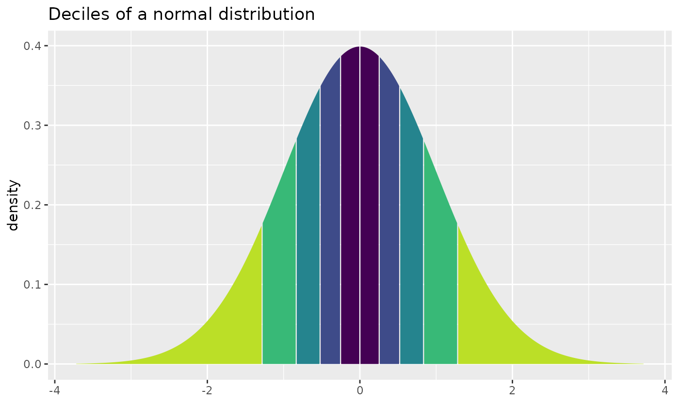 #> [1] -1.2815516 -0.8416212 -0.5244005 -0.2533471 0.0000000 0.2533471 0.5244005
#> [8] 0.8416212 1.2815516
xqnorm(seq(.2, .8, by = 0.20), mean = 100, sd = 10)
#>
#> If X ~ N(100, 10), then
#> P(X <= 91.58379) = 0.2 P(X <= 97.46653) = 0.4 P(X <= 102.53347) = 0.6 P(X <= 108.41621) = 0.8
#> P(X > 91.58379) = 0.8 P(X > 97.46653) = 0.6 P(X > 102.53347) = 0.4 P(X > 108.41621) = 0.2
#>
#> [1] -1.2815516 -0.8416212 -0.5244005 -0.2533471 0.0000000 0.2533471 0.5244005
#> [8] 0.8416212 1.2815516
xqnorm(seq(.2, .8, by = 0.20), mean = 100, sd = 10)
#>
#> If X ~ N(100, 10), then
#> P(X <= 91.58379) = 0.2 P(X <= 97.46653) = 0.4 P(X <= 102.53347) = 0.6 P(X <= 108.41621) = 0.8
#> P(X > 91.58379) = 0.8 P(X > 97.46653) = 0.6 P(X > 102.53347) = 0.4 P(X > 108.41621) = 0.2
#>
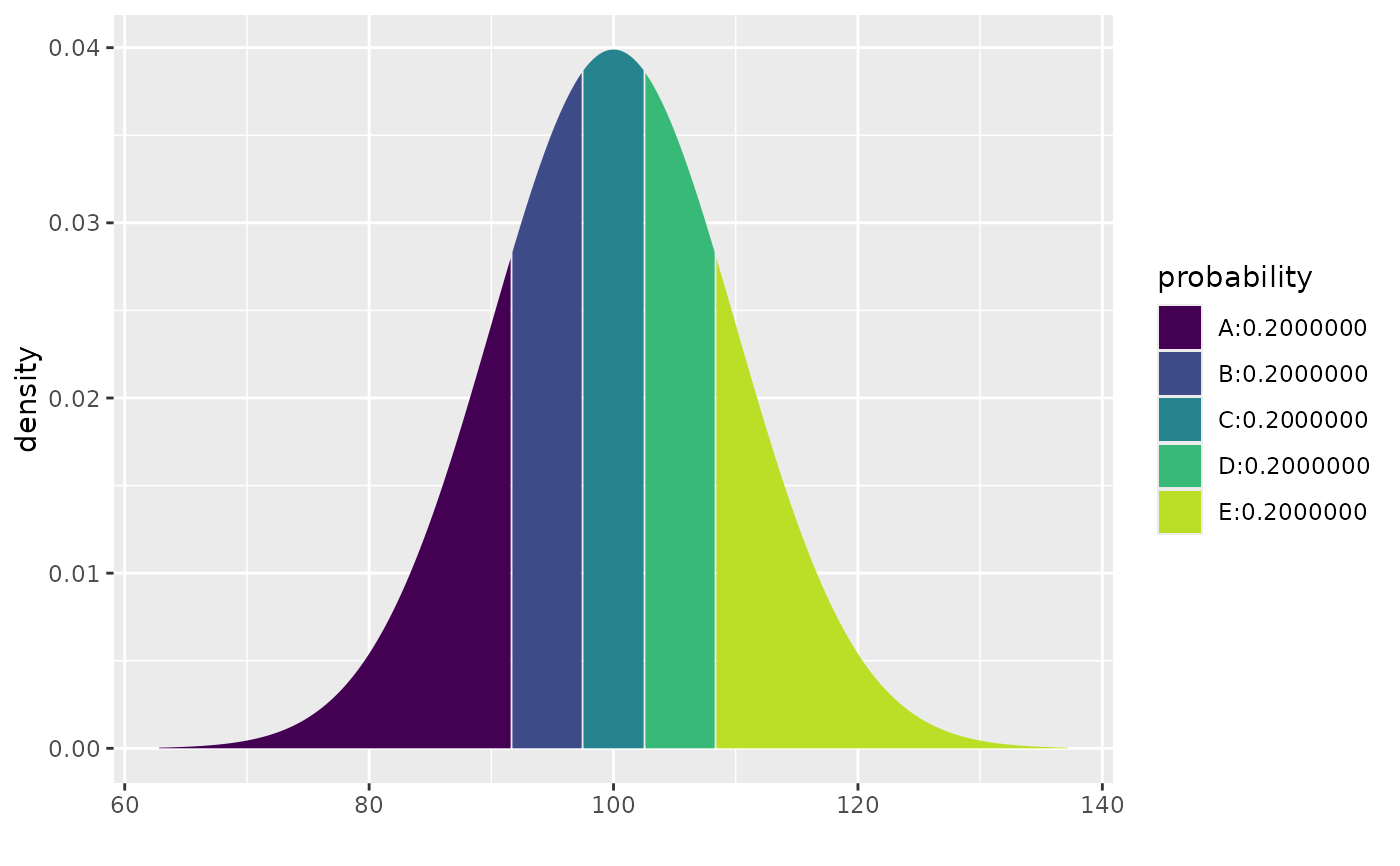 #> [1] 91.58379 97.46653 102.53347 108.41621
qdist("unif", .5)
#> [1] 91.58379 97.46653 102.53347 108.41621
qdist("unif", .5)
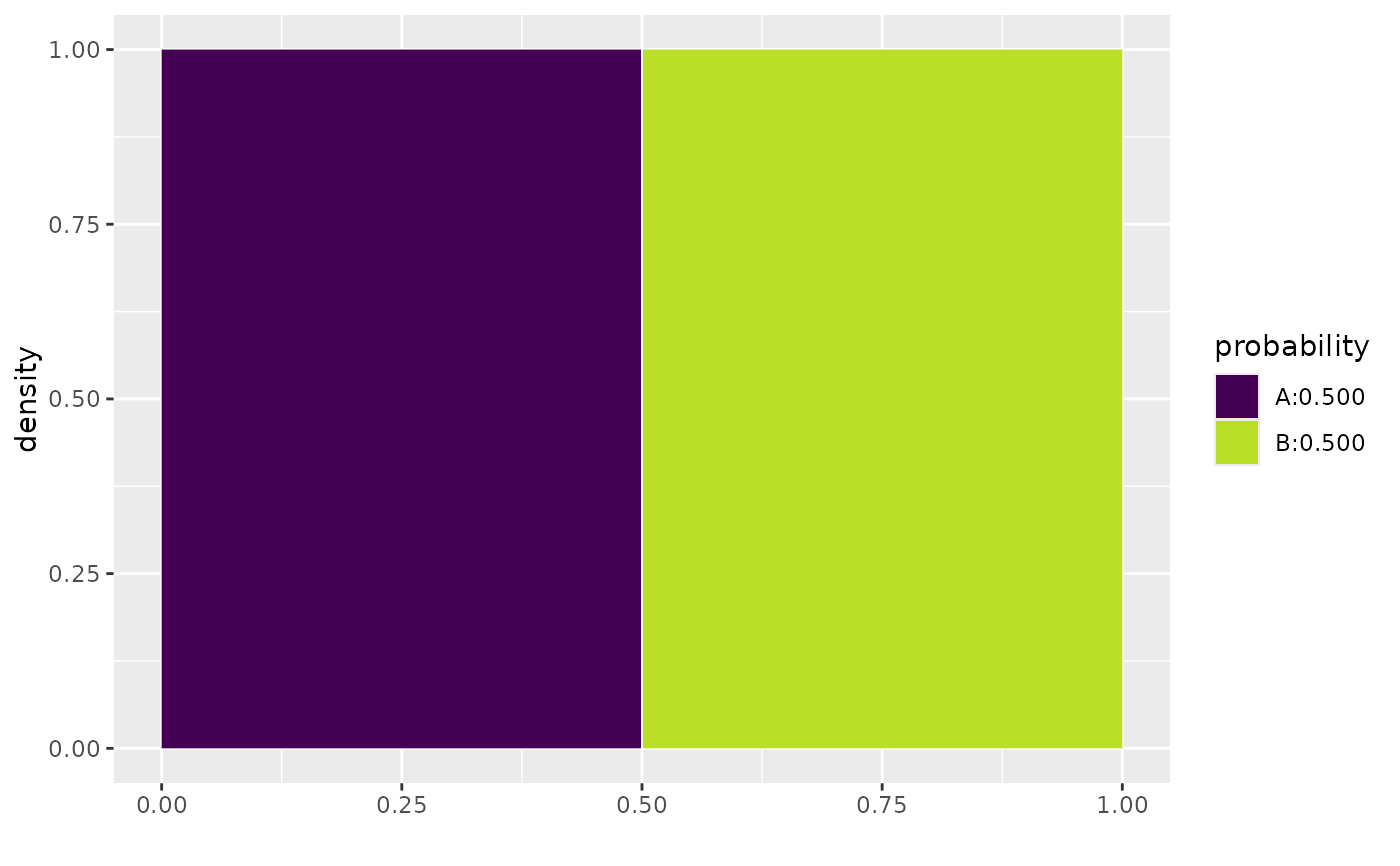 #> [1] 0.5
xqgamma(.5, shape = 3, scale = 4)
#> [1] 0.5
xqgamma(.5, shape = 3, scale = 4)
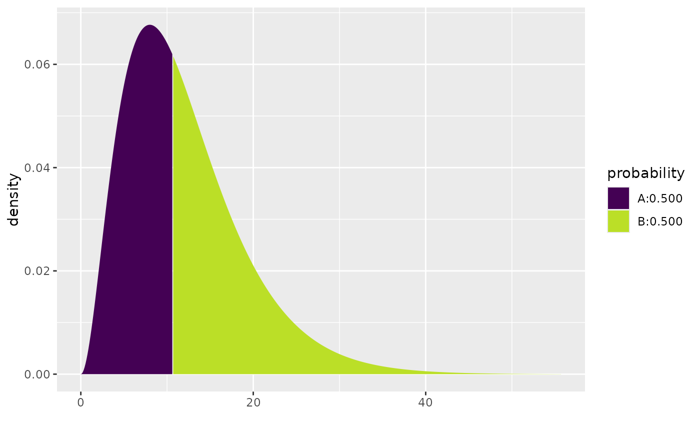 #> [1] 10.69624
xqgamma(.5, shape = 3, scale = 4, color = "black")
#> [1] 10.69624
xqgamma(.5, shape = 3, scale = 4, color = "black")
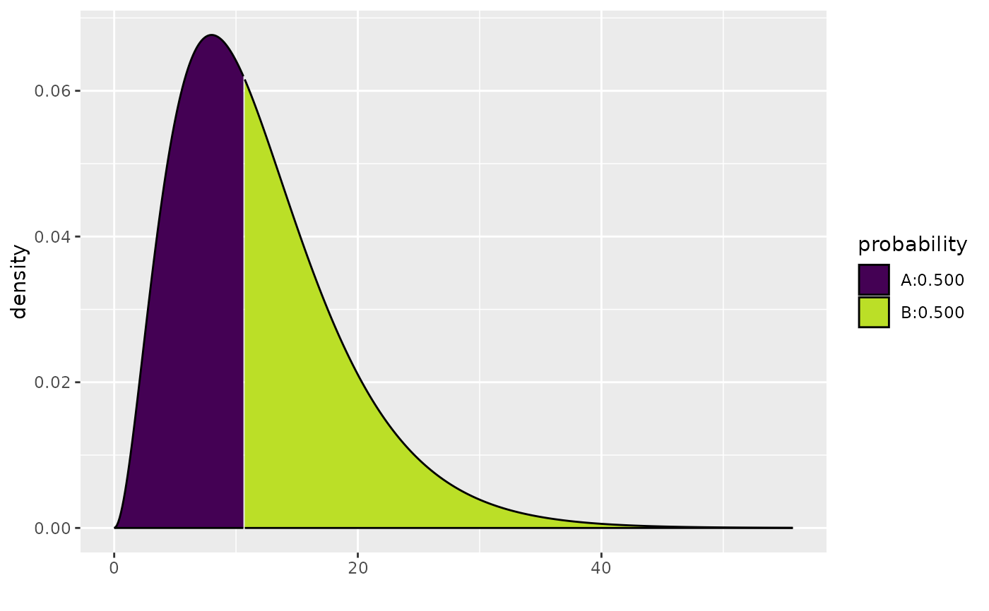 #> [1] 10.69624
xqbeta(.5, shape1 = .9, shape2 = 1.4, dlwd = 1)
#> [1] 10.69624
xqbeta(.5, shape1 = .9, shape2 = 1.4, dlwd = 1)
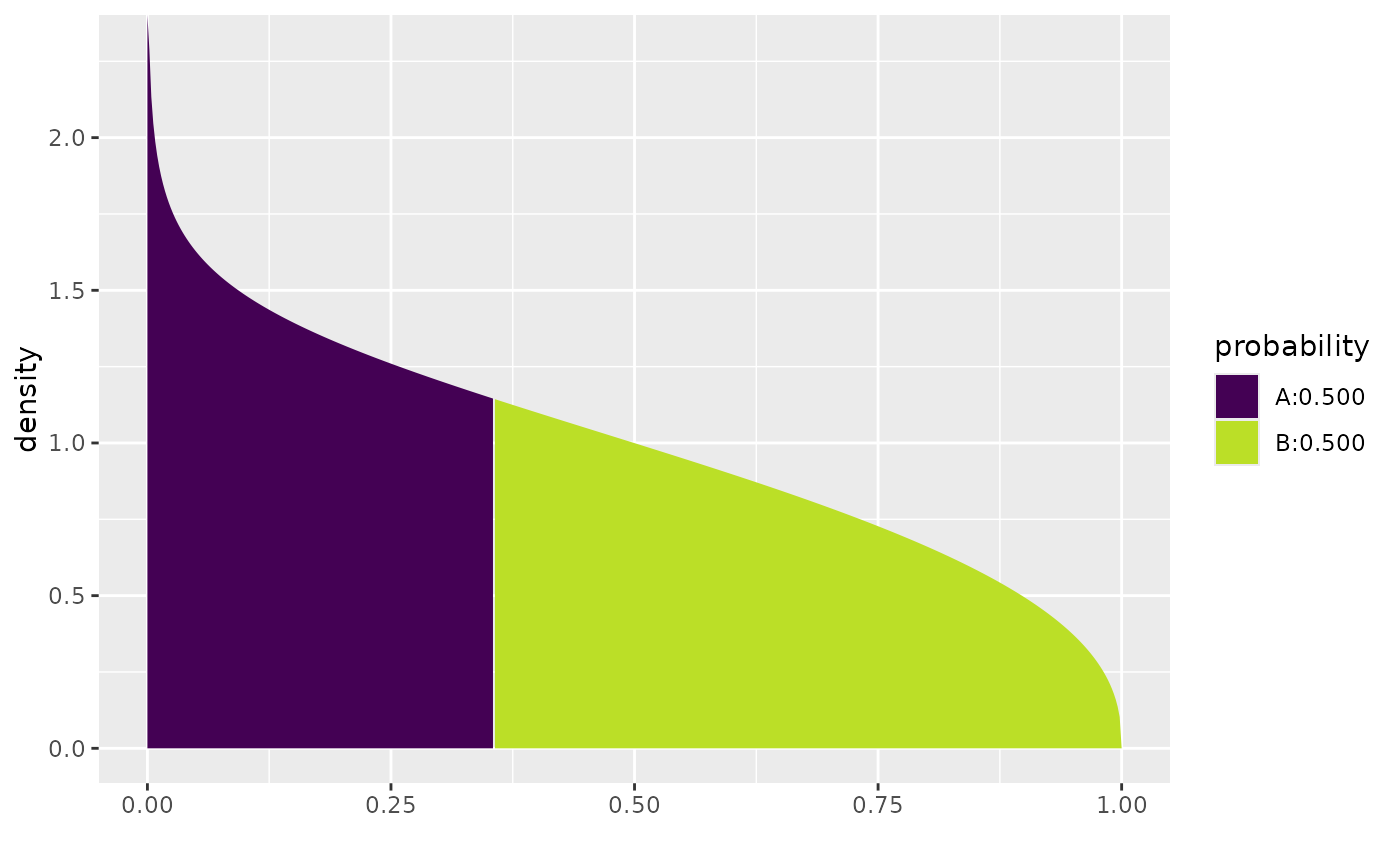 #> [1] 0.3557401
xqchisq(c(.25,.5,.75), df = 3)
#> [1] 0.3557401
xqchisq(c(.25,.5,.75), df = 3)
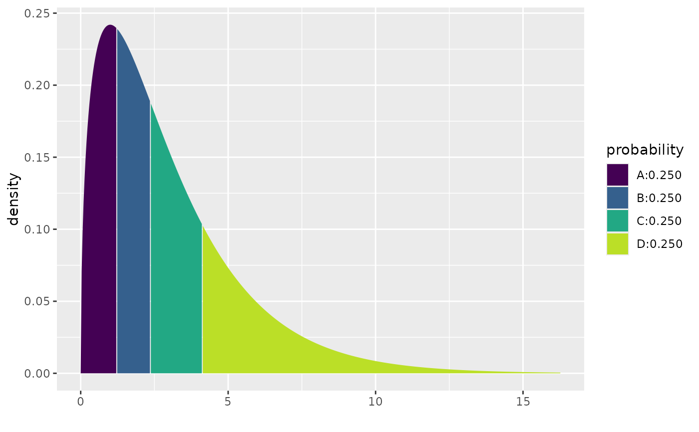 #> [1] 1.212533 2.365974 4.108345
xcbinom(c(0.80, 0.90), size = 1000, prob = 0.40)
#> [1] 1.212533 2.365974 4.108345
xcbinom(c(0.80, 0.90), size = 1000, prob = 0.40)
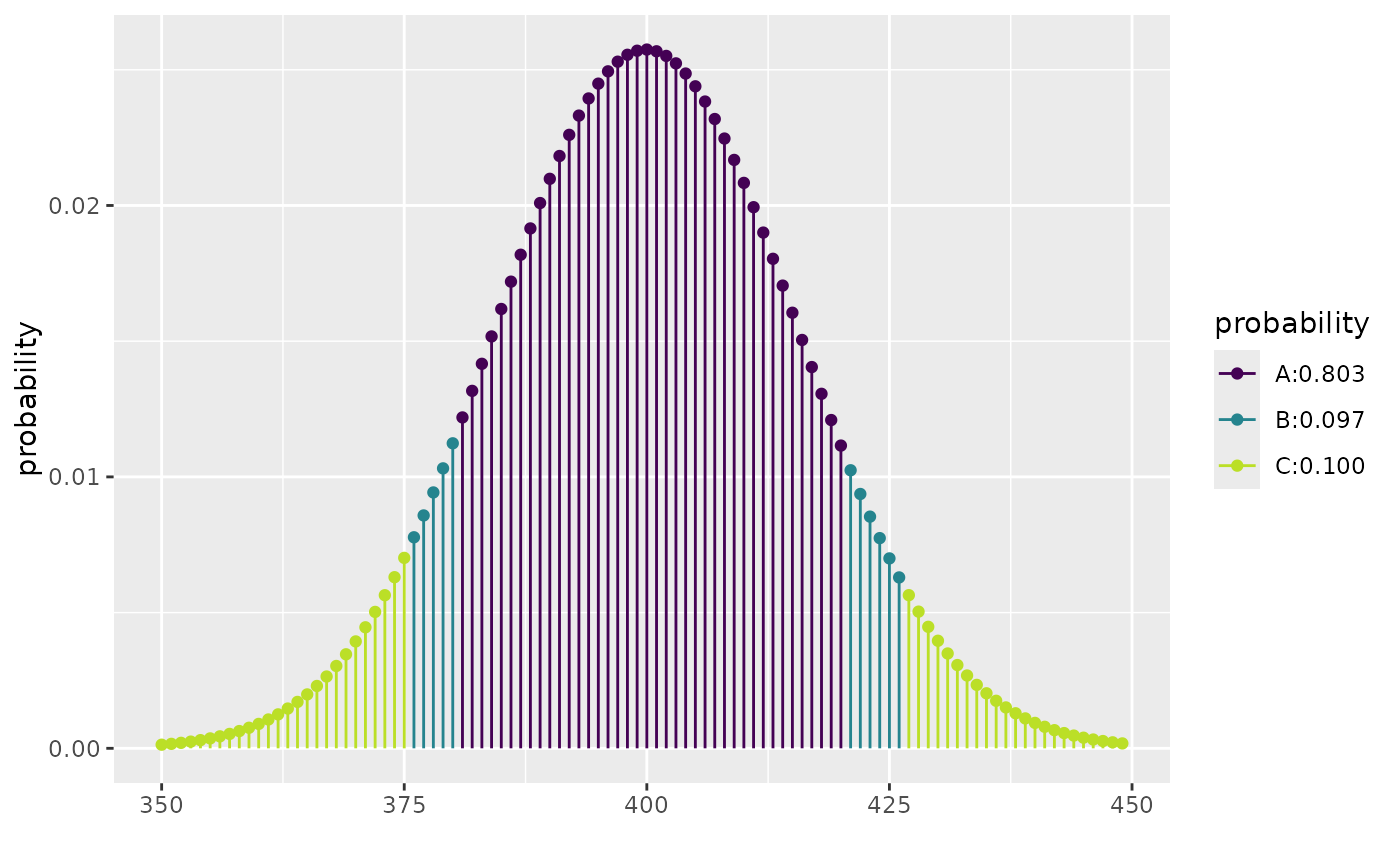 #> [1] 375 380 420 426
# displayed as if continuous
xcbinom(c(0.80, 0.90), size = 5000, prob = 0.40)
#> [1] 375 380 420 426
# displayed as if continuous
xcbinom(c(0.80, 0.90), size = 5000, prob = 0.40)
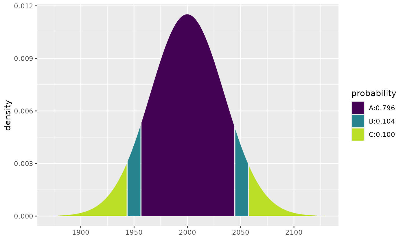 #> [1] 1943 1956 2044 2057
xpbinom(c(480, 500, 520), size = 1000, prob = 0.48)
#> [1] 1943 1956 2044 2057
xpbinom(c(480, 500, 520), size = 1000, prob = 0.48)
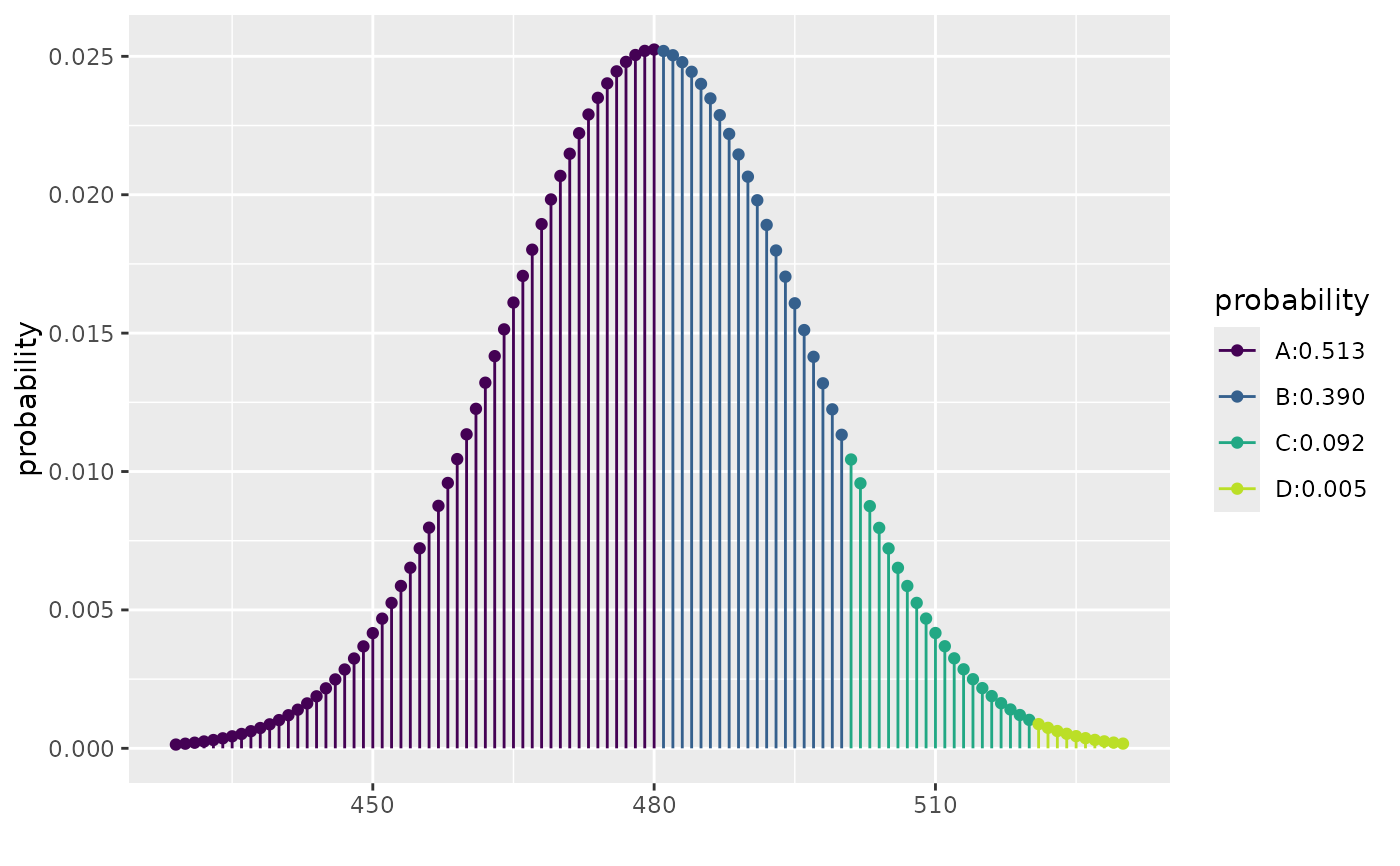 #> [1] 0.5127908 0.9027460 0.9948015
xpbinom(c(40, 60), size = 100, prob = 0.5)
#> [1] 0.5127908 0.9027460 0.9948015
xpbinom(c(40, 60), size = 100, prob = 0.5)
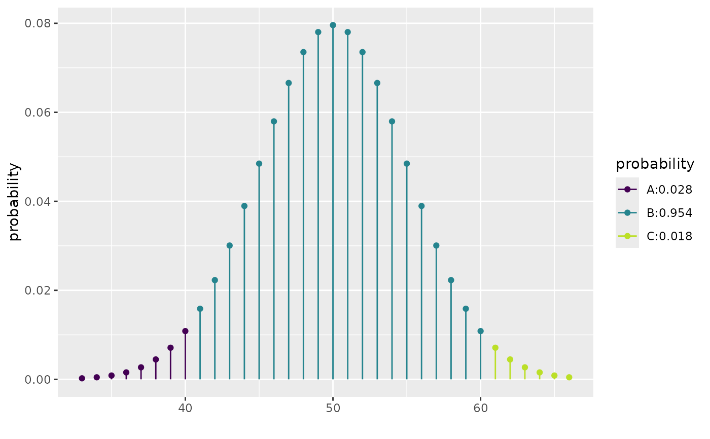 #> [1] 0.02844397 0.98239990
xqpois(c(0.25, 0.5, 0.75), lambda = 12)
#> [1] 0.02844397 0.98239990
xqpois(c(0.25, 0.5, 0.75), lambda = 12)
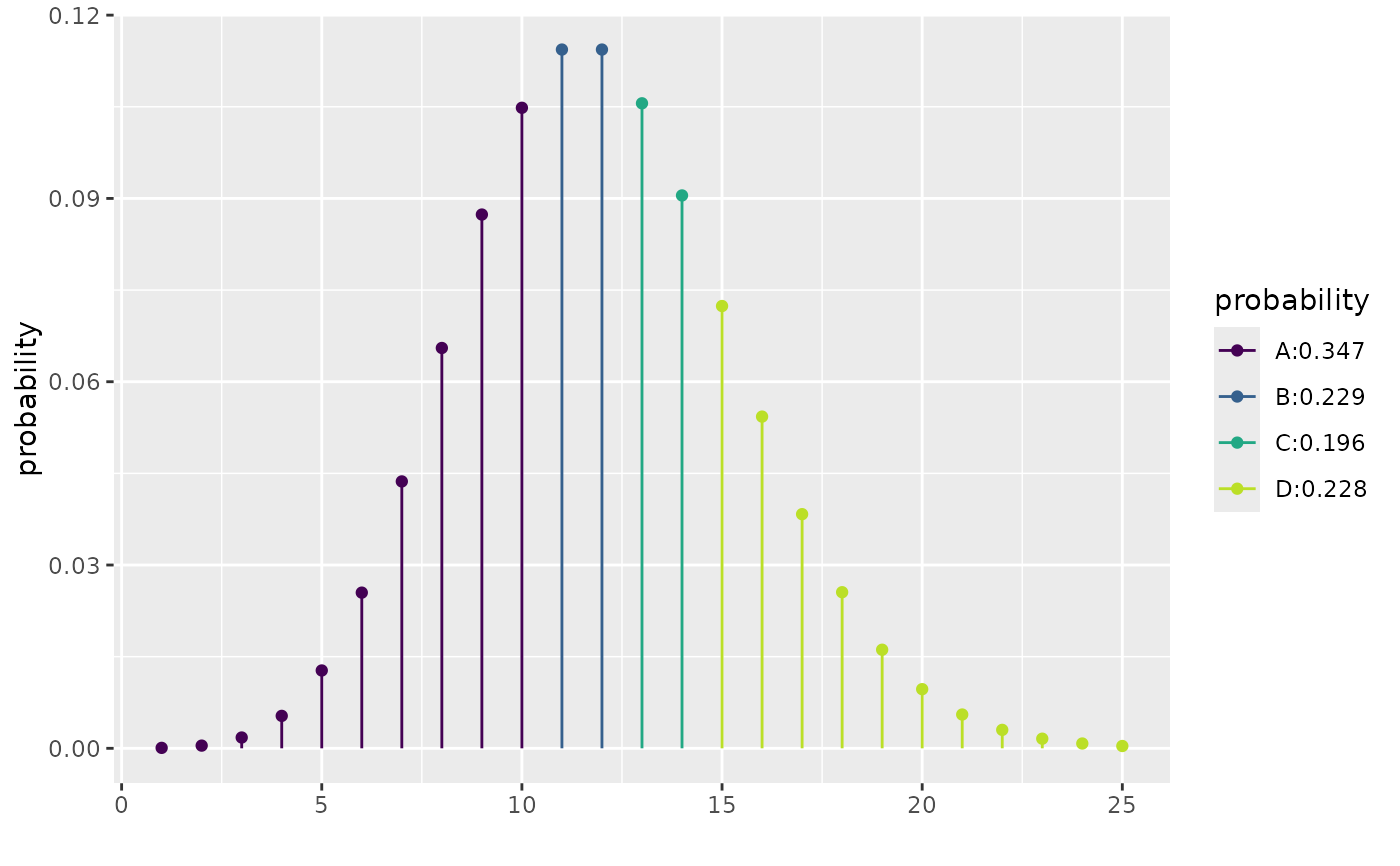 #> [1] 10 12 14
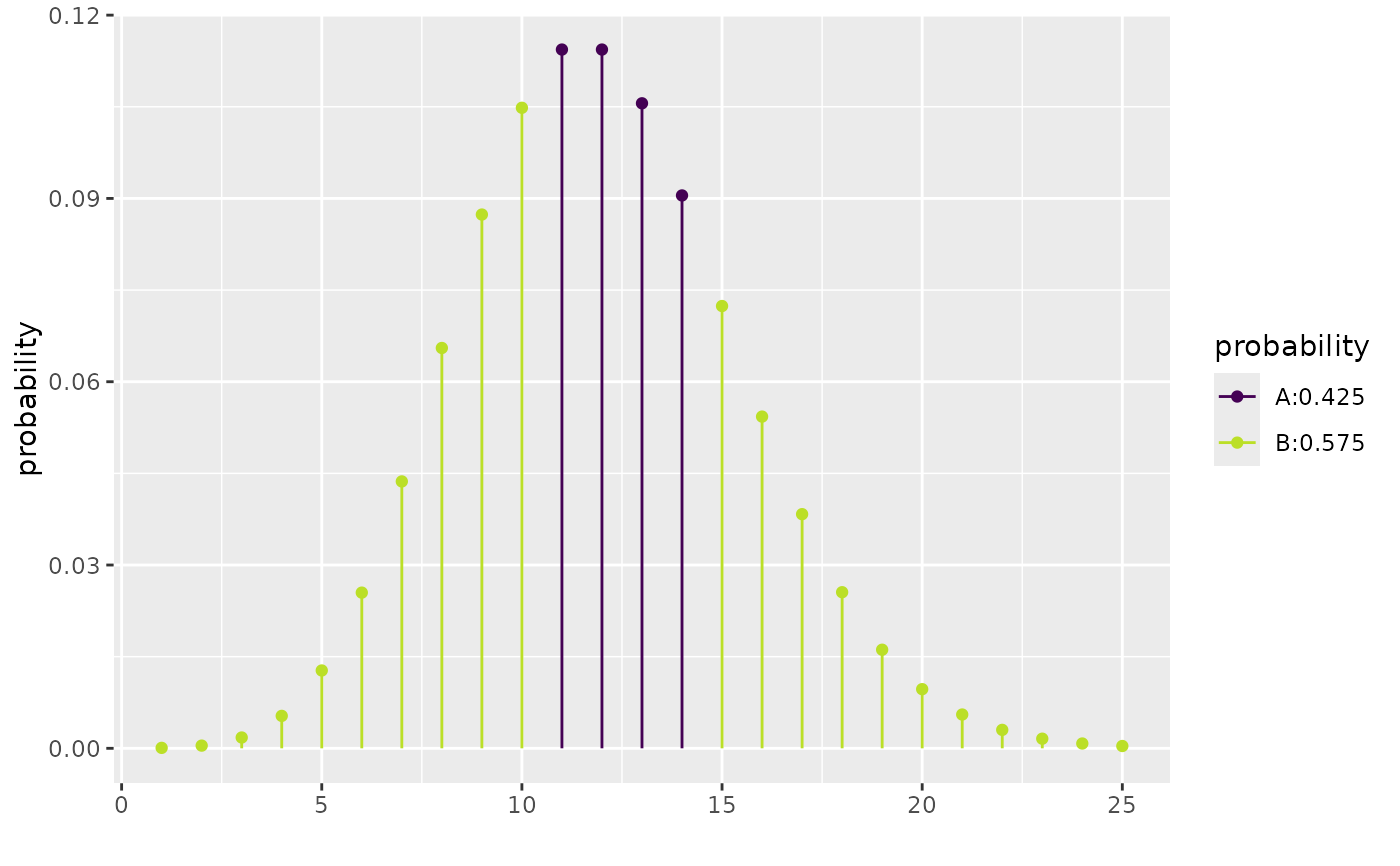
xcpois(0.50, lambda = 12)
#> [1] 10 12 14
xcpois(0.50, lambda = 12)
 #> [1] 10 14
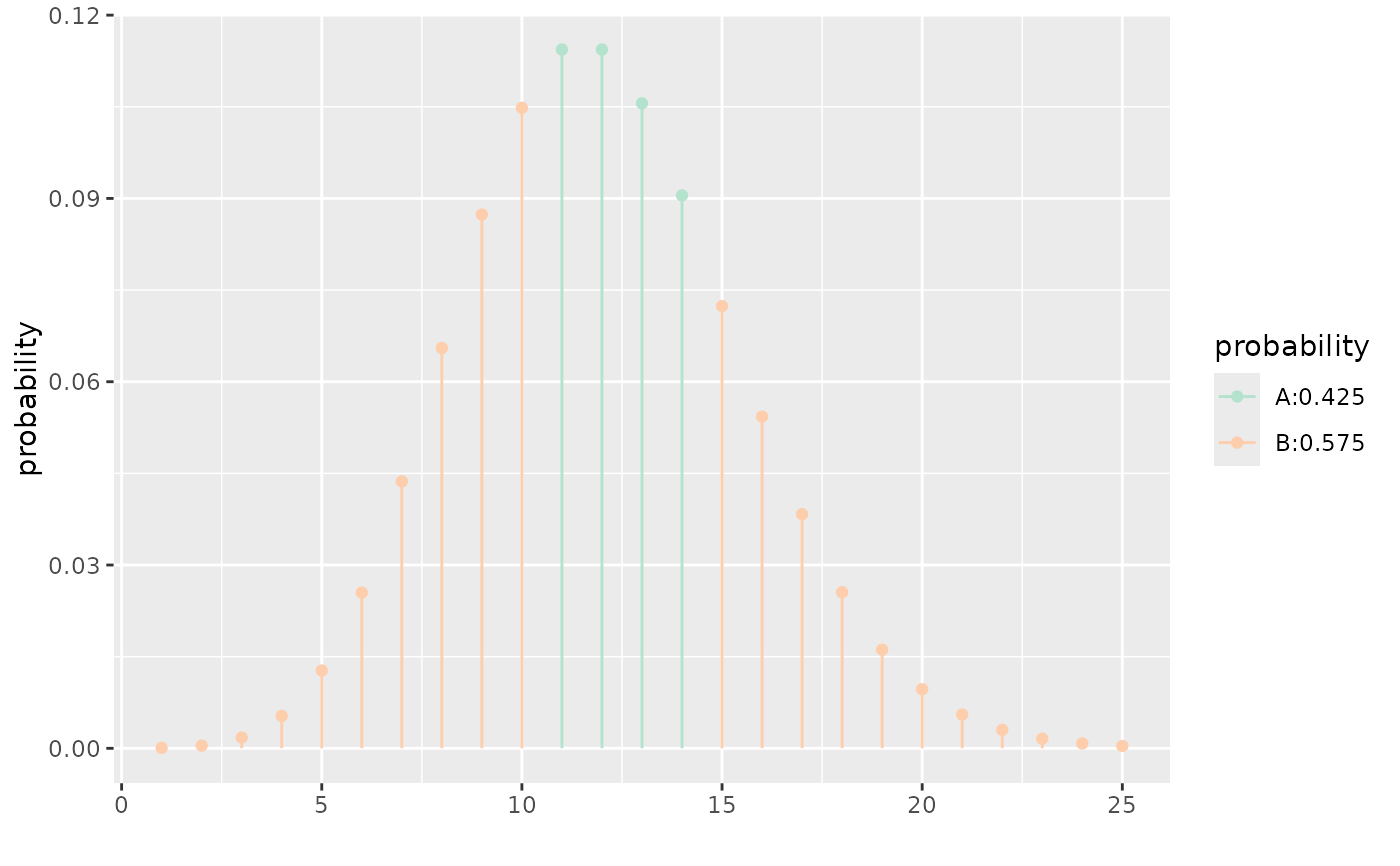
xcpois(0.50, lambda = 12, refinements = list(scale_color_brewer(type = "qual", palette = 5)))
#> Scale for colour is already present.
#> Adding another scale for colour, which will replace the existing scale.
#> [1] 10 14
xcpois(0.50, lambda = 12, refinements = list(scale_color_brewer(type = "qual", palette = 5)))
#> Scale for colour is already present.
#> Adding another scale for colour, which will replace the existing scale.
 #> [1] 10 14