Return residuals of a DHARMa simulation
Usage
# S3 method for class 'DHARMa'
residuals(object, quantileFunction = NULL,
  outlierValues = NULL, ...)
Arguments
- object
an object with simulated residuals created by simulateResiduals.
- quantileFunction
optional - a quantile function to transform the uniform 0/1 scaling of DHARMa to another distribution.
- outlierValues
if a quantile function with infinite support (such as dnorm) is used, residuals that are 0/1 are mapped to -Inf / Inf. outlierValues allows to convert -Inf / Inf values to an optional min / max value.
- ...
optional arguments for compatibility with the generic function, no function implemented.
Details
The function accesses the slot $scaledResiduals in a fitted DHARMa object, and optionally transforms the standard DHARMa quantile residuals (which have a uniform distribution) to a particular pdf.
Note
Some of the papers on simulated quantile residuals transforming the residuals (which are natively uniform) back to a normal distribution. I presume this is because of the larger familiarity of most users with normal residuals. Personally, I never considered this desirable, for the reasons explained in https://github.com/florianhartig/DHARMa/issues/39, but with this function, I wanted to give users the option to plot normal residuals if they so wish.
Examples
library(lme4)
testData = createData(sampleSize = 100, overdispersion = 0.5, family = poisson())
fittedModel <- glmer(observedResponse ~ Environment1 + (1|group),
family = "poisson", data = testData)
# simulate residuals (default behavior, conditional on the fitted random effects)
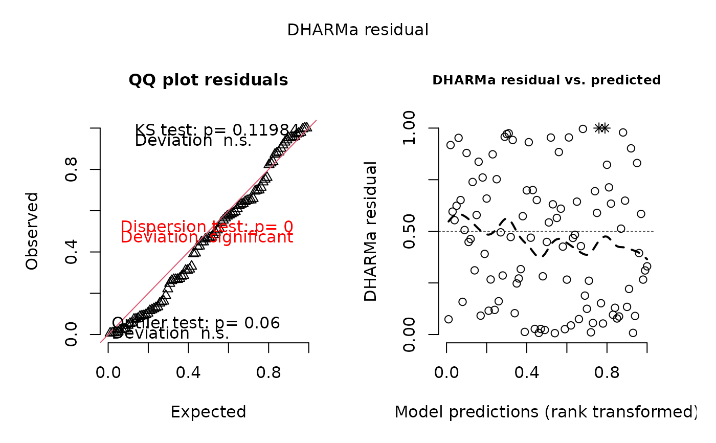
simulationOutput1 <- simulateResiduals(fittedModel = fittedModel)
plot(simulationOutput1, quantreg = FALSE)
 # simulate residuals unconditional on the fitted random effects (REs are re-simulated)
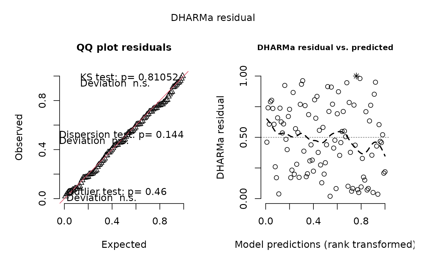
simulationOutput2 <- simulateResiduals(fittedModel = fittedModel,
simulateREs = "unconditional")
plot(simulationOutput2, quantreg = FALSE)
# simulate residuals unconditional on the fitted random effects (REs are re-simulated)
simulationOutput2 <- simulateResiduals(fittedModel = fittedModel,
simulateREs = "unconditional")
plot(simulationOutput2, quantreg = FALSE)
 # simulate residuals user-specified using lme4 syntax (e.g. conditional only on a specific RE)
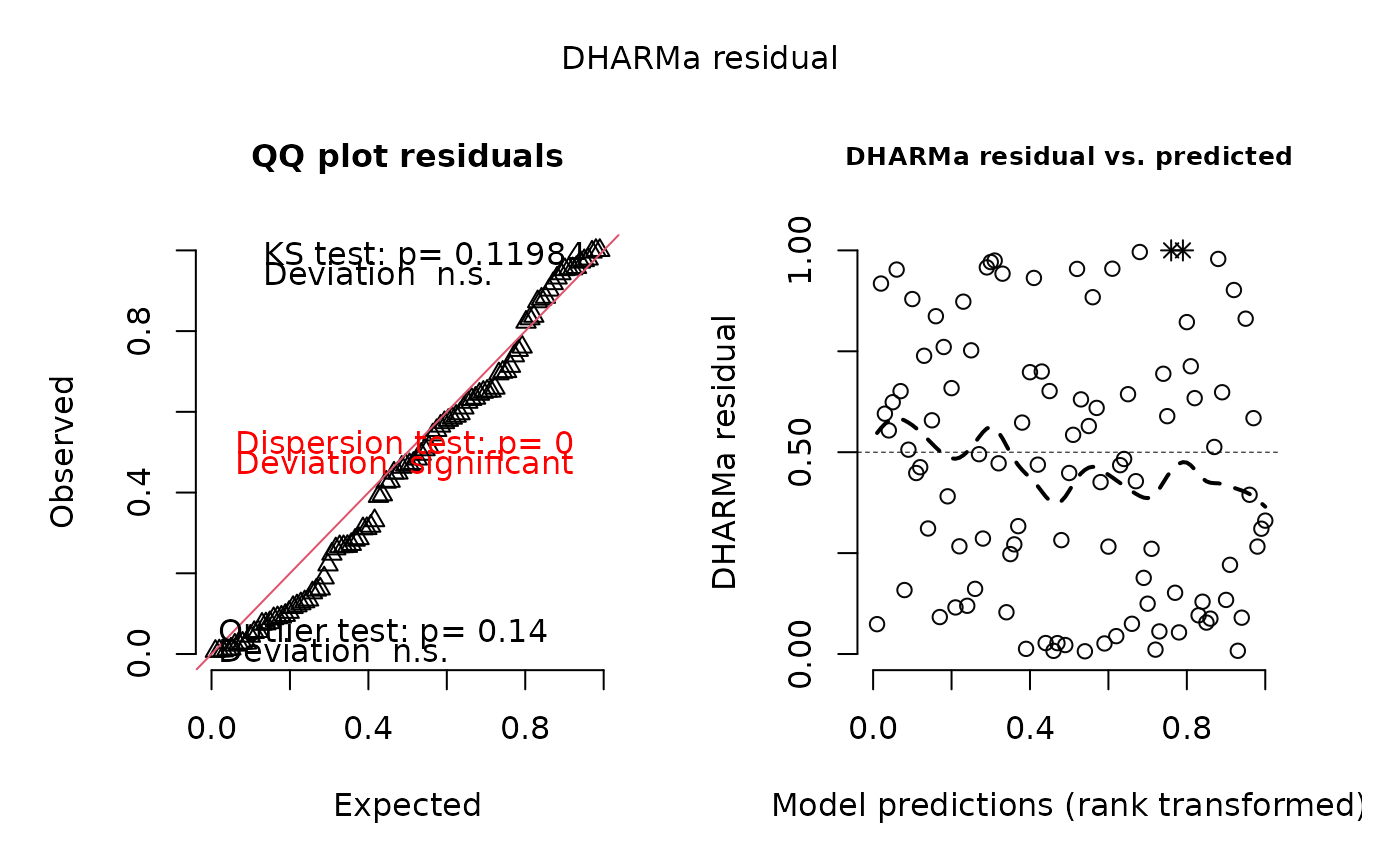
simulationOutput3 <- simulateResiduals(fittedModel = fittedModel,
simulateREs = "user-specified",
re.form = ~(1|group))
plot(simulationOutput3, quantreg = FALSE)
# simulate residuals user-specified using lme4 syntax (e.g. conditional only on a specific RE)
simulationOutput3 <- simulateResiduals(fittedModel = fittedModel,
simulateREs = "user-specified",
re.form = ~(1|group))
plot(simulationOutput3, quantreg = FALSE)
 # one of the possible test, for other options see ?testResiduals / vignette
testDispersion(simulationOutput1)
# one of the possible test, for other options see ?testResiduals / vignette
testDispersion(simulationOutput1)
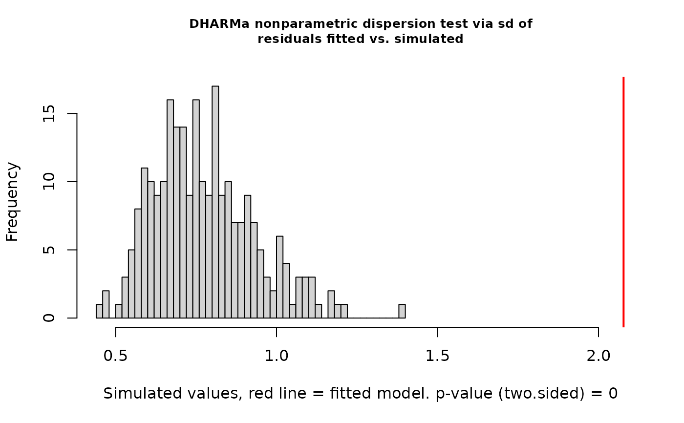 #>
#> DHARMa nonparametric dispersion test via sd of residuals fitted vs.
#> simulated
#>
#> data: simulationOutput
#> dispersion = 2.6776, p-value < 2.2e-16
#> alternative hypothesis: two.sided
#>
# the calculated residuals can be accessed via
residuals(simulationOutput1)
#> [1] 0.564809670 0.271655785 0.266066542 0.462801054 0.158433671 0.007881646
#> [7] 1.000000000 0.124662671 0.220928579 0.008000000 0.584365118 0.006773592
#> [13] 0.954596084 0.055989992 0.394533584 0.589278743 0.483220060 0.942316186
#> [19] 0.310969321 0.651504720 0.090028997 0.077894989 0.448459668 0.879385893
#> [25] 0.633939112 0.760653204 0.698210776 0.188626523 0.822251057 0.012774521
#> [31] 0.883994132 0.428193288 0.495081071 0.247527939 0.022241018 0.651247932
#> [37] 0.630817622 0.266184958 0.694297629 0.573369233 0.917832348 0.310432344
#> [43] 0.161371361 0.978786110 0.316795929 0.425877143 0.087649050 0.330474127
#> [49] 0.648505147 0.830761183 0.469132563 0.260678810 0.974790940 0.954076142
#> [55] 0.872931934 0.836935423 0.623846423 0.266777430 0.010842855 0.512951939
#> [61] 0.074844821 0.553945683 0.129580831 1.000000000 0.390661783 0.282150562
#> [67] 0.699860124 0.119497457 0.901800899 0.044263718 0.103463766 0.073950941
#> [73] 0.095848266 0.658746623 0.578993641 0.995965117 0.091557218 0.971071323
#> [79] 0.643689350 0.026154815 0.595437646 0.467889607 0.134015979 0.952484032
#> [85] 0.286035798 0.448404813 0.712889161 0.609683232 0.506236493 0.027155175
#> [91] 0.543057061 0.752376936 0.053492856 0.738871381 0.931699918 0.027001185
#> [97] 0.957803394 0.151738362 0.115382255 0.472465641
# transform residuals to other pdf, see ?residuals.DHARMa for details
residuals(simulationOutput1, quantileFunction = qnorm, outlierValues = c(-7,7))
#> [1] 0.16317499 -0.60781290 -0.62475315 -0.09337946 -1.00091616 -2.41435048
#> [7] 7.00000000 -1.15198961 -0.76906090 -2.40891555 0.21307333 -2.46905121
#> [13] 1.69115171 -1.58935626 -0.26752214 0.22569003 -0.04207348 1.57451850
#> [19] -0.49310465 0.38938609 -1.34057649 -1.41937410 -0.12955395 1.17192240
#> [25] 0.34230446 0.70840532 0.51926143 -0.88296895 0.92397778 -2.23299851
#> [31] 1.19519274 -0.18097579 -0.01233024 -0.68228955 -2.00951982 0.38869182
#> [37] 0.33401962 -0.62439240 0.50806930 0.18495857 1.39063774 -0.49462523
#> [43] -0.98883736 2.02929964 -0.47667740 -0.18688056 -1.35537504 -0.43860434
#> [49] 0.38128780 0.95717757 -0.07745055 -0.64125408 1.95639943 1.68573051
#> [55] 1.14036052 0.98194051 0.31559866 -0.62258867 -2.29582815 0.03247140
#> [61] -1.44062858 0.13563652 -1.12837481 7.00000000 -0.27759461 -0.57646470
#> [67] 0.52399826 -1.17750272 1.29188145 -1.70321717 -1.26205907 -1.44698230
#> [73] -1.30557674 0.40904484 0.19931964 2.64913679 -1.33122668 1.89677717
#> [79] 0.36833789 -1.94057681 0.24155537 -0.08057592 -1.10760612 1.66943129
#> [85] -0.56500319 -0.12969261 0.56184493 0.27849352 0.01563321 -1.92435302
#> [91] 0.10813844 0.68198865 -1.61189076 0.63986982 1.48857180 -1.92681757
#> [97] 1.72574548 -1.02900628 -1.19839183 -0.06907329
# get residuals that are outside the simulation envelope
outliers(simulationOutput1)
#> [1] 7 64
# calculating aggregated residuals per group
# group here specified as formula (recommended)
# but you can also use a variable from your environment, e.g. testData$group
simulationOutput4 = recalculateResiduals(simulationOutput1, group = ~group)
plot(simulationOutput4, quantreg = FALSE)
#>
#> DHARMa nonparametric dispersion test via sd of residuals fitted vs.
#> simulated
#>
#> data: simulationOutput
#> dispersion = 2.6776, p-value < 2.2e-16
#> alternative hypothesis: two.sided
#>
# the calculated residuals can be accessed via
residuals(simulationOutput1)
#> [1] 0.564809670 0.271655785 0.266066542 0.462801054 0.158433671 0.007881646
#> [7] 1.000000000 0.124662671 0.220928579 0.008000000 0.584365118 0.006773592
#> [13] 0.954596084 0.055989992 0.394533584 0.589278743 0.483220060 0.942316186
#> [19] 0.310969321 0.651504720 0.090028997 0.077894989 0.448459668 0.879385893
#> [25] 0.633939112 0.760653204 0.698210776 0.188626523 0.822251057 0.012774521
#> [31] 0.883994132 0.428193288 0.495081071 0.247527939 0.022241018 0.651247932
#> [37] 0.630817622 0.266184958 0.694297629 0.573369233 0.917832348 0.310432344
#> [43] 0.161371361 0.978786110 0.316795929 0.425877143 0.087649050 0.330474127
#> [49] 0.648505147 0.830761183 0.469132563 0.260678810 0.974790940 0.954076142
#> [55] 0.872931934 0.836935423 0.623846423 0.266777430 0.010842855 0.512951939
#> [61] 0.074844821 0.553945683 0.129580831 1.000000000 0.390661783 0.282150562
#> [67] 0.699860124 0.119497457 0.901800899 0.044263718 0.103463766 0.073950941
#> [73] 0.095848266 0.658746623 0.578993641 0.995965117 0.091557218 0.971071323
#> [79] 0.643689350 0.026154815 0.595437646 0.467889607 0.134015979 0.952484032
#> [85] 0.286035798 0.448404813 0.712889161 0.609683232 0.506236493 0.027155175
#> [91] 0.543057061 0.752376936 0.053492856 0.738871381 0.931699918 0.027001185
#> [97] 0.957803394 0.151738362 0.115382255 0.472465641
# transform residuals to other pdf, see ?residuals.DHARMa for details
residuals(simulationOutput1, quantileFunction = qnorm, outlierValues = c(-7,7))
#> [1] 0.16317499 -0.60781290 -0.62475315 -0.09337946 -1.00091616 -2.41435048
#> [7] 7.00000000 -1.15198961 -0.76906090 -2.40891555 0.21307333 -2.46905121
#> [13] 1.69115171 -1.58935626 -0.26752214 0.22569003 -0.04207348 1.57451850
#> [19] -0.49310465 0.38938609 -1.34057649 -1.41937410 -0.12955395 1.17192240
#> [25] 0.34230446 0.70840532 0.51926143 -0.88296895 0.92397778 -2.23299851
#> [31] 1.19519274 -0.18097579 -0.01233024 -0.68228955 -2.00951982 0.38869182
#> [37] 0.33401962 -0.62439240 0.50806930 0.18495857 1.39063774 -0.49462523
#> [43] -0.98883736 2.02929964 -0.47667740 -0.18688056 -1.35537504 -0.43860434
#> [49] 0.38128780 0.95717757 -0.07745055 -0.64125408 1.95639943 1.68573051
#> [55] 1.14036052 0.98194051 0.31559866 -0.62258867 -2.29582815 0.03247140
#> [61] -1.44062858 0.13563652 -1.12837481 7.00000000 -0.27759461 -0.57646470
#> [67] 0.52399826 -1.17750272 1.29188145 -1.70321717 -1.26205907 -1.44698230
#> [73] -1.30557674 0.40904484 0.19931964 2.64913679 -1.33122668 1.89677717
#> [79] 0.36833789 -1.94057681 0.24155537 -0.08057592 -1.10760612 1.66943129
#> [85] -0.56500319 -0.12969261 0.56184493 0.27849352 0.01563321 -1.92435302
#> [91] 0.10813844 0.68198865 -1.61189076 0.63986982 1.48857180 -1.92681757
#> [97] 1.72574548 -1.02900628 -1.19839183 -0.06907329
# get residuals that are outside the simulation envelope
outliers(simulationOutput1)
#> [1] 7 64
# calculating aggregated residuals per group
# group here specified as formula (recommended)
# but you can also use a variable from your environment, e.g. testData$group
simulationOutput4 = recalculateResiduals(simulationOutput1, group = ~group)
plot(simulationOutput4, quantreg = FALSE)
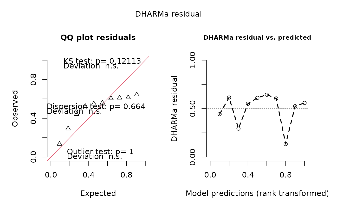 # we see one residual point per RE
# with group as variable in your environment
# but then you need to exclude NAs by hand
simulationOutput5 = recalculateResiduals(simulationOutput1, group = testData$group)
# calculating residuals only for subset of the data
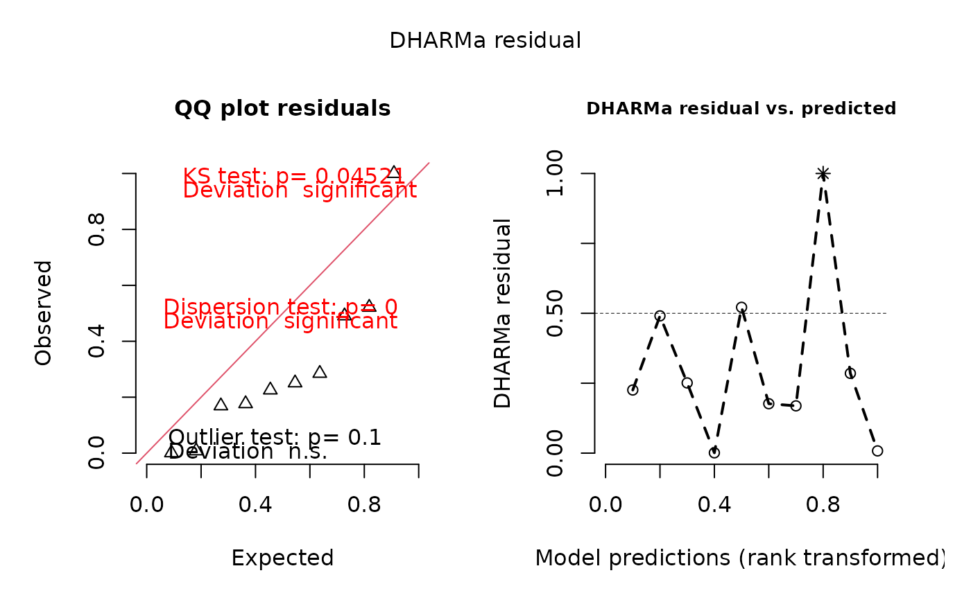
simulationOutput6 = recalculateResiduals(simulationOutput1, sel = testData$group == 1)
plot(simulationOutput6, quantreg = FALSE)
# we see one residual point per RE
# with group as variable in your environment
# but then you need to exclude NAs by hand
simulationOutput5 = recalculateResiduals(simulationOutput1, group = testData$group)
# calculating residuals only for subset of the data
simulationOutput6 = recalculateResiduals(simulationOutput1, sel = testData$group == 1)
plot(simulationOutput6, quantreg = FALSE)
 # or with sel as formula
simulationOutput7 = recalculateResiduals(simulationOutput1, sel = ~Environment1<0.5)
# as condition based on a variable in your environment
simulationOutput8 = recalculateResiduals(simulationOutput1, sel = testData$Environment1<0.5)
# or combine group and sel
simulationOutput9 = recalculateResiduals(simulationOutput1, group = ~group, sel = ~Environment1<0.5)
# or as subset of rows
# (note: order of rows is based on residuals, not on original dataframe)
# so be careful with NAs!
simulationOutput10 = recalculateResiduals(simulationOutput1, sel = 1:20)
# or with sel as formula
simulationOutput7 = recalculateResiduals(simulationOutput1, sel = ~Environment1<0.5)
# as condition based on a variable in your environment
simulationOutput8 = recalculateResiduals(simulationOutput1, sel = testData$Environment1<0.5)
# or combine group and sel
simulationOutput9 = recalculateResiduals(simulationOutput1, group = ~group, sel = ~Environment1<0.5)
# or as subset of rows
# (note: order of rows is based on residuals, not on original dataframe)
# so be careful with NAs!
simulationOutput10 = recalculateResiduals(simulationOutput1, sel = 1:20)