The function creates scaled residuals by simulating from the fitted model. Residuals can be extracted with residuals.DHARMa. See testResiduals for an overview of residual tests, plot.DHARMa for an overview of available plots.
Arguments
- fittedModel
a fitted model of a class supported by DHARMa.
- n
number of simulations. The smaller the number, the higher the stochastic error on the residuals. Also, for very small n, discretization artefacts can influence the tests. Default is 250, which is a relatively safe value. You can consider increasing to 1000 to stabilize the simulated values.
- simulateREs
decides which REs / hierarchical levels should be re-simulated. If
conditional, simulations are done conditional on all fitted random effects (default). Ifunconditional, all REs or hierchical levels are re-simulated. Settinguser-specifiedallows supplying package-specific arguments to decide which REs are to be re-simulated. If none are supplied, the defaults of the respective fitted model object is used. See details and further comments in getSimulations.- refit
if FALSE, new data will be simulated and scaled residuals will be created by comparing observed data with new data. If TRUE, the model will be refitted on the simulated data (parametric bootstrap), and scaled residuals will be created by comparing observed with refitted residuals.
- integerResponse
if TRUE, noise will be added to the residuals to maintain uniform expectations for integer responses (such as Poisson or Binomial). Usually, the model will automatically detect the appropriate setting, so there is no need to adjust this setting.
- plot
if TRUE, plotResiduals will be directly run after the residuals have been calculated.
- seed
the random seed to be used within DHARMa. The default setting, recommended for most users, is to keep the random seed on a fixed value of 123. This means that you will always get the same randomization and thus the same result when running the same code. If NULL, no new seed is set, but previous random state will be restored after simulation. If FALSE, no seed is set, and random state will not be restored. The latter two options are only recommended for simulation experiments. See vignette for details.
- method
for refit = FALSE, the quantile randomization method is used. The two options implemented at the moment are probability integral transform (PIT-) residuals (current default), and the "traditional" randomization procedure, that was used in DHARMa until version 0.3.0. refit = T will always use "traditional", regardless of the value of method. For details, see getQuantile.
- rotation
optional rotation of the residual space prior to calculating the quantile residuals. The main purpose of this is to account for residual covariance as created by temporal, spatial or phylogenetic autocorrelation. See details below, section residual autocorrelation as well as the help of getQuantile and, for a practical example, testTemporalAutocorrelation.
- ...
further parameters to pass on to the simulate and update function of the model object (via DHARMa::getSimulations and DHARMa::getRefit). If simulateREs = "user-specified", an important use of this is to specify whether simulations should be conditional on all, some or none of the current random effect estimates, e.g. via re.form. Note that not all models support syntax to specify conditional or unconditional simulations. See details and getSimulations.
Value
an S3 class of type "DHARMa". Implemented S3 functions include plot.DHARMa, print.DHARMa and residuals.DHARMa. For other functions that can be used on a DHARMa object, see section "See Also" below.
Details
There are a number of important considerations when simulating from a more complex (hierarchical) model:
Re-simulating random effects / hierarchical structure: in a hierarchical or RE model, we have several stochastic processes on top of each other. For example, in a typical Poisson GLMM, we have a lower level normal distribution (random effect), whose result enters at the next hierarchical level into a Poisson distribution. For other hierarchical models such as state-space models, similar considerations apply. When simulating new data in such a situation, we have to decide if we want to re-simulate all stochastic levels (unconditional), only the top level conditional on all other levels (conditional), or if we want to re-simulate a specific subset of REs while conditioning on the others. As of DHARMa 0.5.0, the default was changed to simulating conditionally on all fitted REs. If this is not what you want, you can switch simulateREs to either "unconditional", or "user-specified", which allows to condition on a user-specified set of REs. With "user-specified", if no additional arguments are set, this results in the package behavior previous to version 0.5.0. Note that the syntax to change the behavior is different for each package. Also, specific packages may lack certain functionalities. For further details, please see vignette, getSimulations and refer to the help of the different simulate functions (e.g. ?simulate.merMod). #'
When to use conditional and unconditional simulations: If the model is correctly specified, the simulated residuals should be flat regardless which hierarchical levels you re-simulate. Re-simulating all levels (unconditional) can be advantageous because it tests the model structure as a whole. If REs are correlated with a predictor, for example, this will show up in the residuals. A potential drawback is that re-simulating the lower-level random effects creates more variability and correlation structures in the residuals, which may reduce power for detecting problems in the upper-level stochastic processes and, in some cases, can lead to inflated type I error rates through the induces correlations. In particular dispersion tests may produce different results when switching from conditional to unconditional simulations, and often the conditional simulation is more sensitive. The default was therefore switched to conditional in DHARMa 0.5.0 which we consider to be more safe, but it can make sense to overrule this default for specific tests.
Refitting or not: a third issue is how residuals are calculated. simulateResiduals has two options that are controlled by the refit parameter:
if refit = FALSE (default), new data is simulated from the fitted model, and residuals are calculated by comparing the observed data to the new data.
if refit = TRUE, a parametric bootstrap is performed, meaning that the model is refit on the new data, and residuals are created by comparing observed residuals against refitted residuals. I advise against using this method per default (see more comments in the vignette), unless you are really sure that you need it.
Residuals per group: In many situations, it can be useful to look at residuals per group, e.g. to see how much the model over / underpredicts per plot, year or subject. To do this, use recalculateResiduals, together with a grouping variable (see also help).
Transformation to other distributions: DHARMa calculates residuals for which the theoretical expectation (assuming a correctly specified model) is uniform. To transform these residuals to another distribution (e.g. so that a correctly specified model will have normal residuals) see residuals.DHARMa.
Integer responses: this is only relevant if method = "traditional", in which case it activates the randomization of the residuals. Usually, this does not need to be changed, as DHARMa will try to automatically check if the fitted model has an integer or discrete distribution via the family argument. However, in some cases the family does not allow to uniquely identify the distribution type. For example, a tweedie distribution can be integer or continuous. Therefore, DHARMa will additionally check the simulation results for repeated values, and will change the distribution type if repeated values are found (a message is displayed in this case).
Residual autocorrelation: a common problem is residual autocorrelation. Spatial, temporal and phylogenetic autocorrelation can be tested with testSpatialAutocorrelation, testTemporalAutocorrelation and testPhylogeneticAutocorrelation. If simulations are unconditional, residual correlations will be maintained, even if the autocorrelation is addressed by an appropriate CAR structure. This may be a problem, because autocorrelation may create apparently systematic patterns in plots or tests such as testUniformity. To reduce this problem, either simulate conditional on fitted correlated REs, or rotate residuals via the rotation parameter (the latter will likely only work in approximately linear models). See getQuantile for details on the rotation.
Examples
library(lme4)
testData = createData(sampleSize = 100, overdispersion = 0.5, family = poisson())
fittedModel <- glmer(observedResponse ~ Environment1 + (1|group),
family = "poisson", data = testData)
# simulate residuals (default behavior, conditional on the fitted random effects)
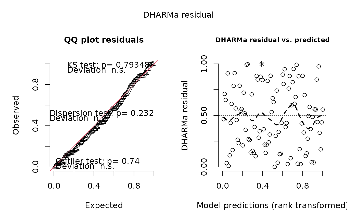
simulationOutput1 <- simulateResiduals(fittedModel = fittedModel)
plot(simulationOutput1, quantreg = FALSE)
 # simulate residuals unconditional on the fitted random effects (REs are re-simulated)
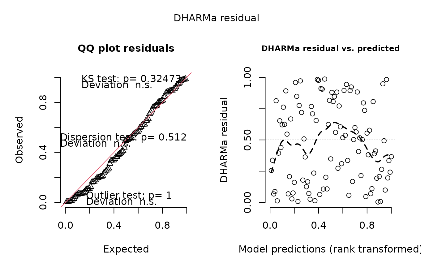
simulationOutput2 <- simulateResiduals(fittedModel = fittedModel,
simulateREs = "unconditional")
plot(simulationOutput2, quantreg = FALSE)
# simulate residuals unconditional on the fitted random effects (REs are re-simulated)
simulationOutput2 <- simulateResiduals(fittedModel = fittedModel,
simulateREs = "unconditional")
plot(simulationOutput2, quantreg = FALSE)
 # simulate residuals user-specified using lme4 syntax (e.g. conditional only on a specific RE)
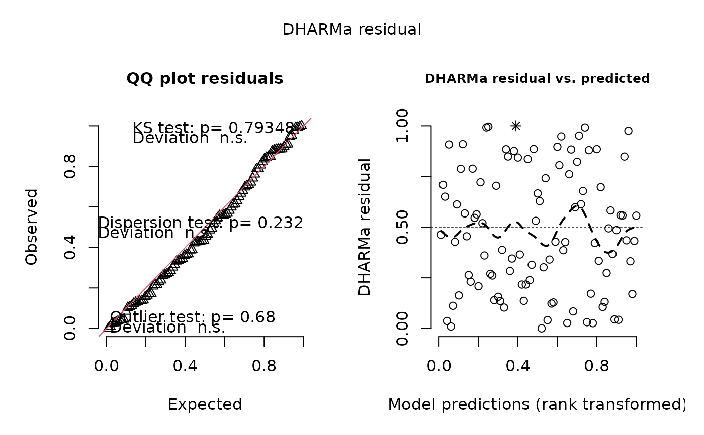
simulationOutput3 <- simulateResiduals(fittedModel = fittedModel,
simulateREs = "user-specified",
re.form = ~(1|group))
plot(simulationOutput3, quantreg = FALSE)
# simulate residuals user-specified using lme4 syntax (e.g. conditional only on a specific RE)
simulationOutput3 <- simulateResiduals(fittedModel = fittedModel,
simulateREs = "user-specified",
re.form = ~(1|group))
plot(simulationOutput3, quantreg = FALSE)
 # one of the possible test, for other options see ?testResiduals / vignette
testDispersion(simulationOutput1)
# one of the possible test, for other options see ?testResiduals / vignette
testDispersion(simulationOutput1)
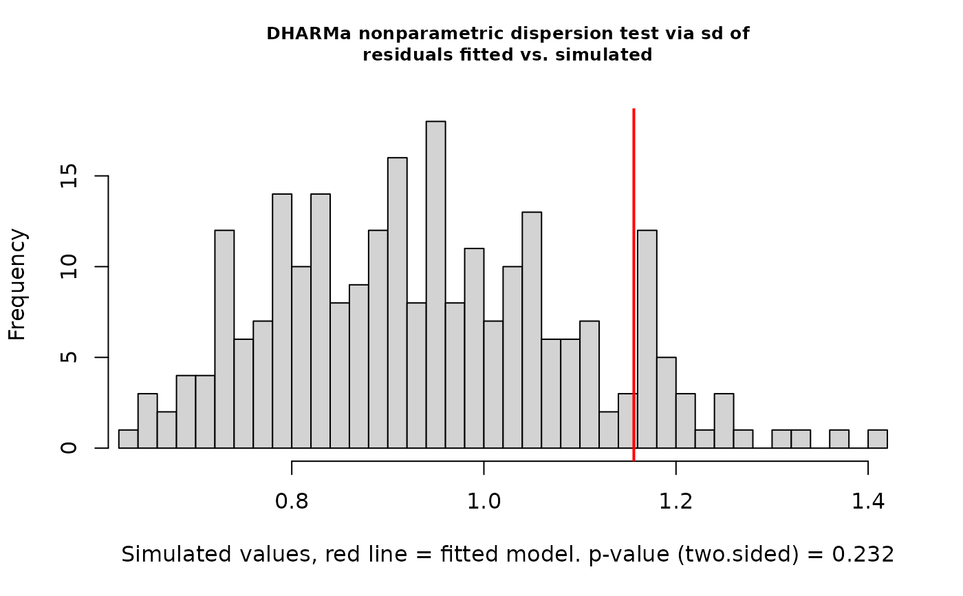 #>
#> DHARMa nonparametric dispersion test via sd of residuals fitted vs.
#> simulated
#>
#> data: simulationOutput
#> dispersion = 1.23, p-value = 0.232
#> alternative hypothesis: two.sided
#>
# the calculated residuals can be accessed via
residuals(simulationOutput1)
#> [1] 0.9960000000 0.1229454477 0.6130317091 0.7607176207 0.5676975917
#> [6] 0.3020523474 0.0263162987 0.5195639399 0.8828192678 0.2740230199
#> [11] 0.4548562756 0.4350949692 0.9917057702 0.4217676825 0.2308055967
#> [16] 0.0098435387 0.0446823697 0.0430017599 0.2637465098 0.6661572807
#> [21] 0.3144469645 0.4263640344 0.7874811085 0.9512615320 0.1356849106
#> [26] 0.2384530666 0.0840749051 0.8852145807 0.5566380014 0.3675030862
#> [31] 0.6970347402 0.0312142122 0.9093949804 0.4940335252 0.3339657585
#> [36] 0.1699594183 0.6119037852 0.6778906377 0.8481794213 0.7410625606
#> [41] 0.1061170712 0.6502205465 0.4627571699 0.4321092990 0.8794315580
#> [46] 0.2612448732 0.8845910078 0.3317117896 0.5456107559 0.8961700340
#> [51] 0.1362495978 0.5573166105 0.9752611208 0.8355880734 0.7209826393
#> [56] 0.3861732213 0.0006987677 0.0412672759 0.2167861288 0.8431348453
#> [61] 0.3403139974 0.2168953172 0.8480033524 0.5820994945 0.2084175783
#> [66] 0.3452691605 0.2839385649 0.9077335145 0.1561830395 0.8755081986
#> [71] 0.7882969633 0.0269722158 0.7085780924 0.5981376677 0.3650646858
#> [76] 0.8220964668 0.0371461046 0.1119575799 0.8840644309 0.4282401327
#> [81] 0.5631270599 0.1314492992 0.9474798044 0.4854279428 0.1032019215
#> [86] 0.3876456647 0.9920001638 0.7039401133 0.3603038809 0.5587070958
#> [91] 0.5312758115 0.4275073956 0.1716682312 0.1395734426 0.6282891082
#> [96] 0.8052220624 0.2699144186 0.1630018845 1.0000000000 0.1284722865
# transform residuals to other pdf, see ?residuals.DHARMa for details
residuals(simulationOutput1, quantileFunction = qnorm, outlierValues = c(-7,7))
#> [1] 2.65206981 -1.16038794 0.28722952 0.70861285 0.17051541 -0.51850683
#> [7] -1.93792316 0.04905920 1.18919876 -0.60069066 -0.11340112 -0.16341723
#> [13] 2.39570446 -0.19737337 -0.73619638 -2.33225886 -1.69875827 -1.71686676
#> [19] -0.63183757 0.42932677 -0.48328424 -0.18563874 0.79771175 1.65721044
#> [25] -1.09991348 -0.71128744 -1.37817323 1.20146509 0.14245073 -0.33847379
#> [31] 0.51589103 -1.86324059 1.33703859 -0.01495629 -0.42898861 -0.95432563
#> [37] 0.28428441 0.46180840 1.02865642 0.64662468 -1.24744563 0.38591596
#> [43] -0.09348994 -0.17100657 1.17214989 -0.63951225 1.19825442 -0.43519130
#> [49] 0.11457943 1.26002614 -1.09732534 0.14416930 1.96445148 0.97648566
#> [55] 0.58576310 -0.28930702 -3.19515958 -1.73616563 -0.78309342 1.00742557
#> [61] -0.41160633 -0.78272157 1.02790760 0.20726743 -0.81192415 -0.39812463
#> [67] -0.57118074 1.32692658 -1.01026973 1.15282163 0.80052606 -1.92728251
#> [73] 0.54923554 0.24852961 -0.34495344 0.92338412 -1.78480958 -1.21618315
#> [79] 1.19555275 -0.18085643 0.15890226 -1.11956636 1.62089392 -0.03653486
#> [85] -1.26351588 -0.28546054 2.40892302 0.53576674 -0.35764665 0.14769205
#> [91] 0.07847731 -0.18272374 -0.94759345 -1.08223778 0.32732540 0.86042307
#> [97] -0.61307184 -0.98219504 7.00000000 -1.13364242
# get residuals that are outside the simulation envelope
outliers(simulationOutput1)
#> [1] 99
# calculating aggregated residuals per group
# group here specified as formula (recommended)
# but you can also use a variable from your environment, e.g. testData$group
simulationOutput4 = recalculateResiduals(simulationOutput1, group = ~group)
plot(simulationOutput4, quantreg = FALSE)
#>
#> DHARMa nonparametric dispersion test via sd of residuals fitted vs.
#> simulated
#>
#> data: simulationOutput
#> dispersion = 1.23, p-value = 0.232
#> alternative hypothesis: two.sided
#>
# the calculated residuals can be accessed via
residuals(simulationOutput1)
#> [1] 0.9960000000 0.1229454477 0.6130317091 0.7607176207 0.5676975917
#> [6] 0.3020523474 0.0263162987 0.5195639399 0.8828192678 0.2740230199
#> [11] 0.4548562756 0.4350949692 0.9917057702 0.4217676825 0.2308055967
#> [16] 0.0098435387 0.0446823697 0.0430017599 0.2637465098 0.6661572807
#> [21] 0.3144469645 0.4263640344 0.7874811085 0.9512615320 0.1356849106
#> [26] 0.2384530666 0.0840749051 0.8852145807 0.5566380014 0.3675030862
#> [31] 0.6970347402 0.0312142122 0.9093949804 0.4940335252 0.3339657585
#> [36] 0.1699594183 0.6119037852 0.6778906377 0.8481794213 0.7410625606
#> [41] 0.1061170712 0.6502205465 0.4627571699 0.4321092990 0.8794315580
#> [46] 0.2612448732 0.8845910078 0.3317117896 0.5456107559 0.8961700340
#> [51] 0.1362495978 0.5573166105 0.9752611208 0.8355880734 0.7209826393
#> [56] 0.3861732213 0.0006987677 0.0412672759 0.2167861288 0.8431348453
#> [61] 0.3403139974 0.2168953172 0.8480033524 0.5820994945 0.2084175783
#> [66] 0.3452691605 0.2839385649 0.9077335145 0.1561830395 0.8755081986
#> [71] 0.7882969633 0.0269722158 0.7085780924 0.5981376677 0.3650646858
#> [76] 0.8220964668 0.0371461046 0.1119575799 0.8840644309 0.4282401327
#> [81] 0.5631270599 0.1314492992 0.9474798044 0.4854279428 0.1032019215
#> [86] 0.3876456647 0.9920001638 0.7039401133 0.3603038809 0.5587070958
#> [91] 0.5312758115 0.4275073956 0.1716682312 0.1395734426 0.6282891082
#> [96] 0.8052220624 0.2699144186 0.1630018845 1.0000000000 0.1284722865
# transform residuals to other pdf, see ?residuals.DHARMa for details
residuals(simulationOutput1, quantileFunction = qnorm, outlierValues = c(-7,7))
#> [1] 2.65206981 -1.16038794 0.28722952 0.70861285 0.17051541 -0.51850683
#> [7] -1.93792316 0.04905920 1.18919876 -0.60069066 -0.11340112 -0.16341723
#> [13] 2.39570446 -0.19737337 -0.73619638 -2.33225886 -1.69875827 -1.71686676
#> [19] -0.63183757 0.42932677 -0.48328424 -0.18563874 0.79771175 1.65721044
#> [25] -1.09991348 -0.71128744 -1.37817323 1.20146509 0.14245073 -0.33847379
#> [31] 0.51589103 -1.86324059 1.33703859 -0.01495629 -0.42898861 -0.95432563
#> [37] 0.28428441 0.46180840 1.02865642 0.64662468 -1.24744563 0.38591596
#> [43] -0.09348994 -0.17100657 1.17214989 -0.63951225 1.19825442 -0.43519130
#> [49] 0.11457943 1.26002614 -1.09732534 0.14416930 1.96445148 0.97648566
#> [55] 0.58576310 -0.28930702 -3.19515958 -1.73616563 -0.78309342 1.00742557
#> [61] -0.41160633 -0.78272157 1.02790760 0.20726743 -0.81192415 -0.39812463
#> [67] -0.57118074 1.32692658 -1.01026973 1.15282163 0.80052606 -1.92728251
#> [73] 0.54923554 0.24852961 -0.34495344 0.92338412 -1.78480958 -1.21618315
#> [79] 1.19555275 -0.18085643 0.15890226 -1.11956636 1.62089392 -0.03653486
#> [85] -1.26351588 -0.28546054 2.40892302 0.53576674 -0.35764665 0.14769205
#> [91] 0.07847731 -0.18272374 -0.94759345 -1.08223778 0.32732540 0.86042307
#> [97] -0.61307184 -0.98219504 7.00000000 -1.13364242
# get residuals that are outside the simulation envelope
outliers(simulationOutput1)
#> [1] 99
# calculating aggregated residuals per group
# group here specified as formula (recommended)
# but you can also use a variable from your environment, e.g. testData$group
simulationOutput4 = recalculateResiduals(simulationOutput1, group = ~group)
plot(simulationOutput4, quantreg = FALSE)
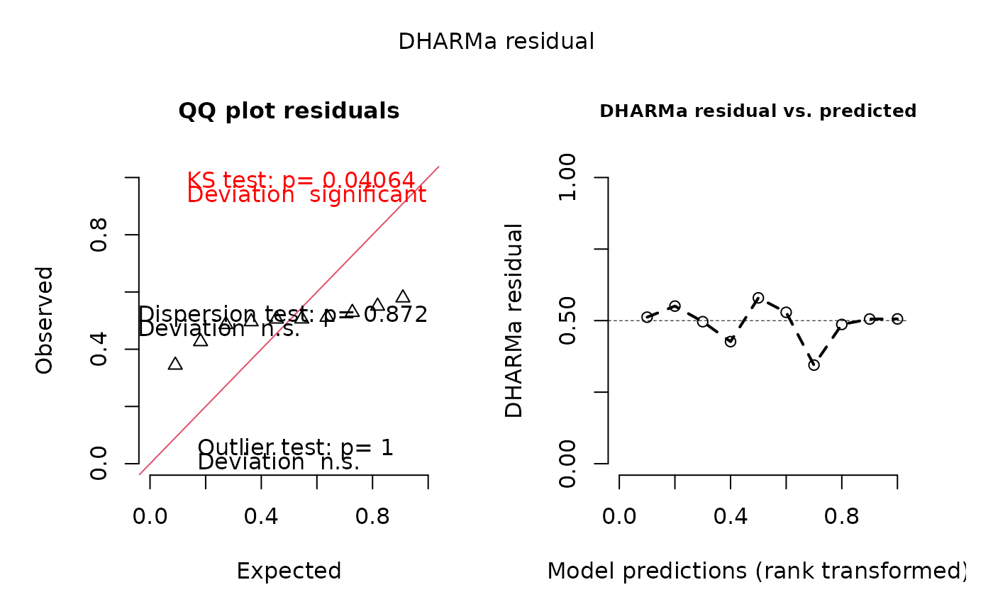 # we see one residual point per RE
# with group as variable in your environment
# but then you need to exclude NAs by hand
simulationOutput5 = recalculateResiduals(simulationOutput1, group = testData$group)
# calculating residuals only for subset of the data
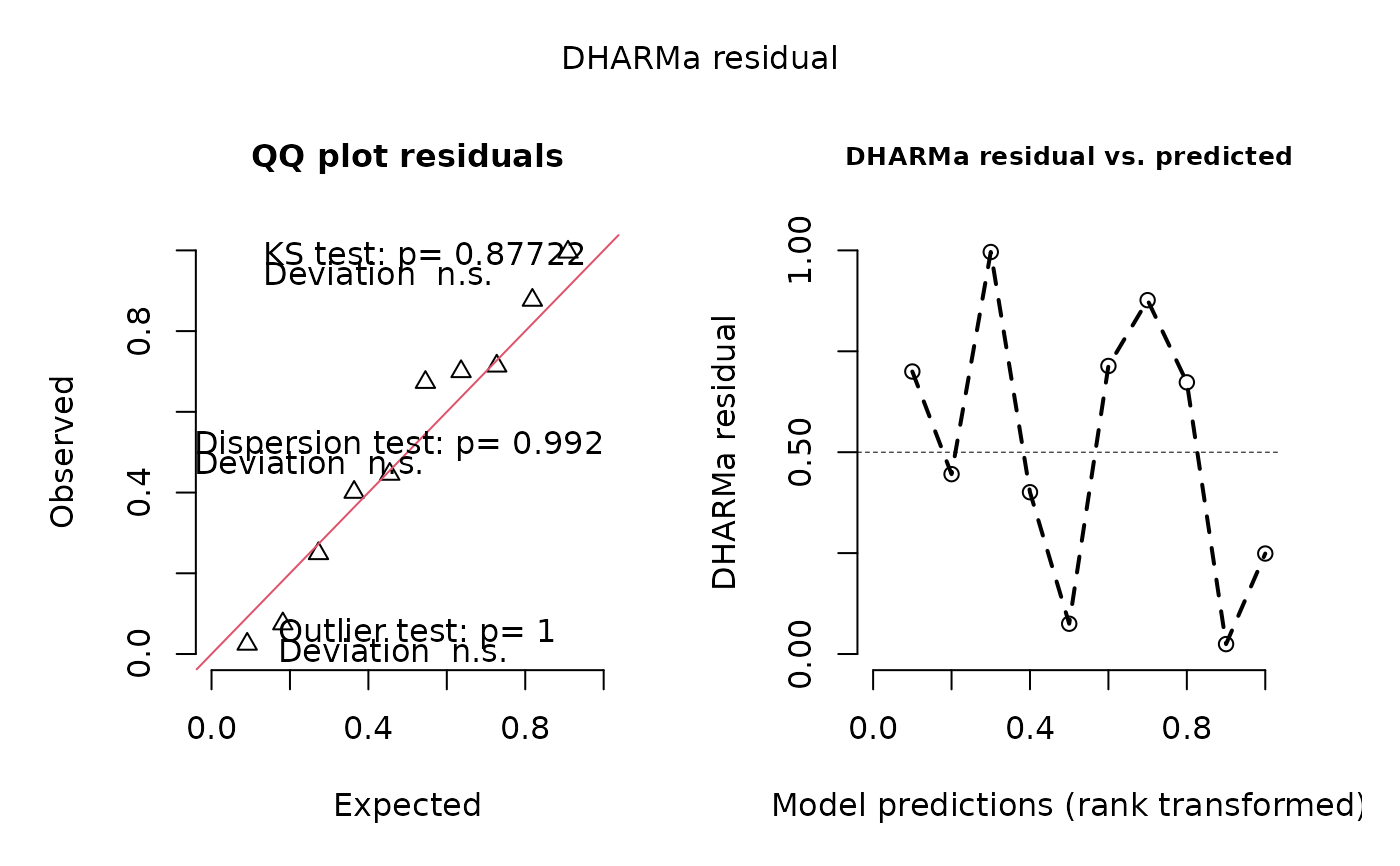
simulationOutput6 = recalculateResiduals(simulationOutput1, sel = testData$group == 1)
plot(simulationOutput6, quantreg = FALSE)
# we see one residual point per RE
# with group as variable in your environment
# but then you need to exclude NAs by hand
simulationOutput5 = recalculateResiduals(simulationOutput1, group = testData$group)
# calculating residuals only for subset of the data
simulationOutput6 = recalculateResiduals(simulationOutput1, sel = testData$group == 1)
plot(simulationOutput6, quantreg = FALSE)
 # or with sel as formula
simulationOutput7 = recalculateResiduals(simulationOutput1, sel = ~Environment1<0.5)
# as condition based on a variable in your environment
simulationOutput8 = recalculateResiduals(simulationOutput1, sel = testData$Environment1<0.5)
# or combine group and sel
simulationOutput9 = recalculateResiduals(simulationOutput1, group = ~group, sel = ~Environment1<0.5)
# or as subset of rows
# (note: order of rows is based on residuals, not on original dataframe)
# so be careful with NAs!
simulationOutput10 = recalculateResiduals(simulationOutput1, sel = 1:20)
# or with sel as formula
simulationOutput7 = recalculateResiduals(simulationOutput1, sel = ~Environment1<0.5)
# as condition based on a variable in your environment
simulationOutput8 = recalculateResiduals(simulationOutput1, sel = testData$Environment1<0.5)
# or combine group and sel
simulationOutput9 = recalculateResiduals(simulationOutput1, group = ~group, sel = ~Environment1<0.5)
# or as subset of rows
# (note: order of rows is based on residuals, not on original dataframe)
# so be careful with NAs!
simulationOutput10 = recalculateResiduals(simulationOutput1, sel = 1:20)