Plot a Raster* object
plot.RdPlot (that is, make a map of) the values of a Raster* object, or make a scatterplot of their values.
Points, lines, and polygons can be drawn on top of a map using plot(..., add=TRUE), or with functions like points, lines, polygons
See the rasterVis package for more advanced (trellis/lattice) plotting of Raster* objects.
Usage
# S4 method for class 'Raster,ANY'
plot(x, y, maxpixels=500000, col, alpha=NULL,
   colNA=NA, add=FALSE, ext=NULL, useRaster=TRUE, interpolate=FALSE,
   addfun=NULL, nc, nr, maxnl=16, main, npretty=0, ...)


# S4 method for class 'Raster,Raster'
plot(x, y, maxpixels=100000, cex, xlab, ylab, nc, nr,
    maxnl=16, main, add=FALSE, gridded=FALSE, ncol=25, nrow=25, ...)
Arguments
- x
Raster* object
- y
If
xis a RasterStack or RasterBrick: integer, character (layer name(s)), or missing to select which layer(s) to plot. If missing, all RasterLayers in the RasterStack will be plotted (up to a maximum of 16). Or another Raster* object of the same extent and resolution, to produce a scatter plot of the cell values.- maxpixels
integer > 0. Maximum number of cells to use for the plot. If
maxpixels < ncell(x),sampleRegularis used before plotting. Ifgridded=TRUEmaxpixels may be ignored to get a larger sample- col
A color palette, i.e. a vector of n contiguous colors generated by functions like rainbow, heat.colors, topo.colors, bpy.colors or one or your own making, perhaps using
colorRampPalette. If none is provided,rev(terrain.colors(255))is used unlessxhas a 'color table'- alpha
Number between 0 and 1 to set transparency. 0 is entirely transparent, 1 is not transparent (NULL is equivalent to 1)
- colNA
The color to use for the background (default is transparent)
- add
Logical. Add to current plot?
- ext
An extent object to zoom in a region (see also
zoomandcrop(x, drawExtent())- useRaster
If
TRUE, the rasterImage function is used for plotting. Otherwise the image function is used. This can be useful if rasterImage does not work well on your system (see note)- interpolate
Logical. Should the image be interpolated (smoothed)? Only used when
useRaster = TRUE- addfun
Function to add additional items such as points or polygons to the plot (map). Typically containing statements like "points(xy); plot(polygons, add=TRUE)". This is particularly useful to add something to each map when plotting a multi-layer Raster* object.
- npretty
integer. Number of decimals for pretty lables on the axes
- ...
Graphical parameters. Any argument that can be passed to
image.plotand to baseplot, such as axes=FALSE, main='title', ylab='latitude'- xlab
Optional. x-axis label)
- ylab
Optional. y-axis label)
- nc
Optional. The number of columns to divide the plotting device in (when plotting multiple layers in a RasterLayer or RasterBrick object)
- nr
Optional. The number of rows to divide the plotting device in (when plotting multiple layers in a RasterLayer or RasterBrick object)
- maxnl
integer. Maximum number of layers to plot (for a multi-layer object)
- main
character. Main plot title
- cex
Symbol size for scatter plots
- gridded
logical. If
TRUEthe scatterplot is gridded (counts by cells)- ncol
integer. Number of columns for gridding
- nrow
integer. Number of rows for gridding
Details
Most of the code for the plot function for a single Raster* object was taken from image.plot (fields package).
Raster objects with a color-table (e.g. a graphics file) are plotted according to that color table.
Note
raster uses rasterImage from the graphics package. For unknown reasons this does not work on Windows Server and on a few versions of Windows XP. On that system you may need to use argument useRaster=FALSE to get a plot.
Examples
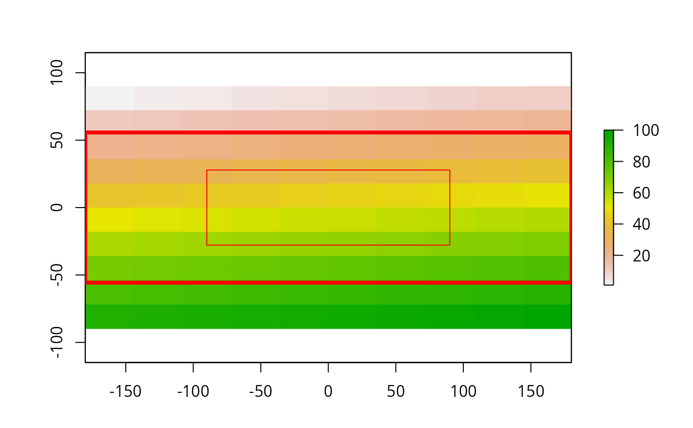
# RasterLayer
r <- raster(nrows=10, ncols=10)
r <- setValues(r, 1:ncell(r))
plot(r)
e <- extent(r)
plot(e, add=TRUE, col='red', lwd=4)
e <- e / 2
plot(e, add=TRUE, col='red')
 # Scatterplot of 2 RasterLayers
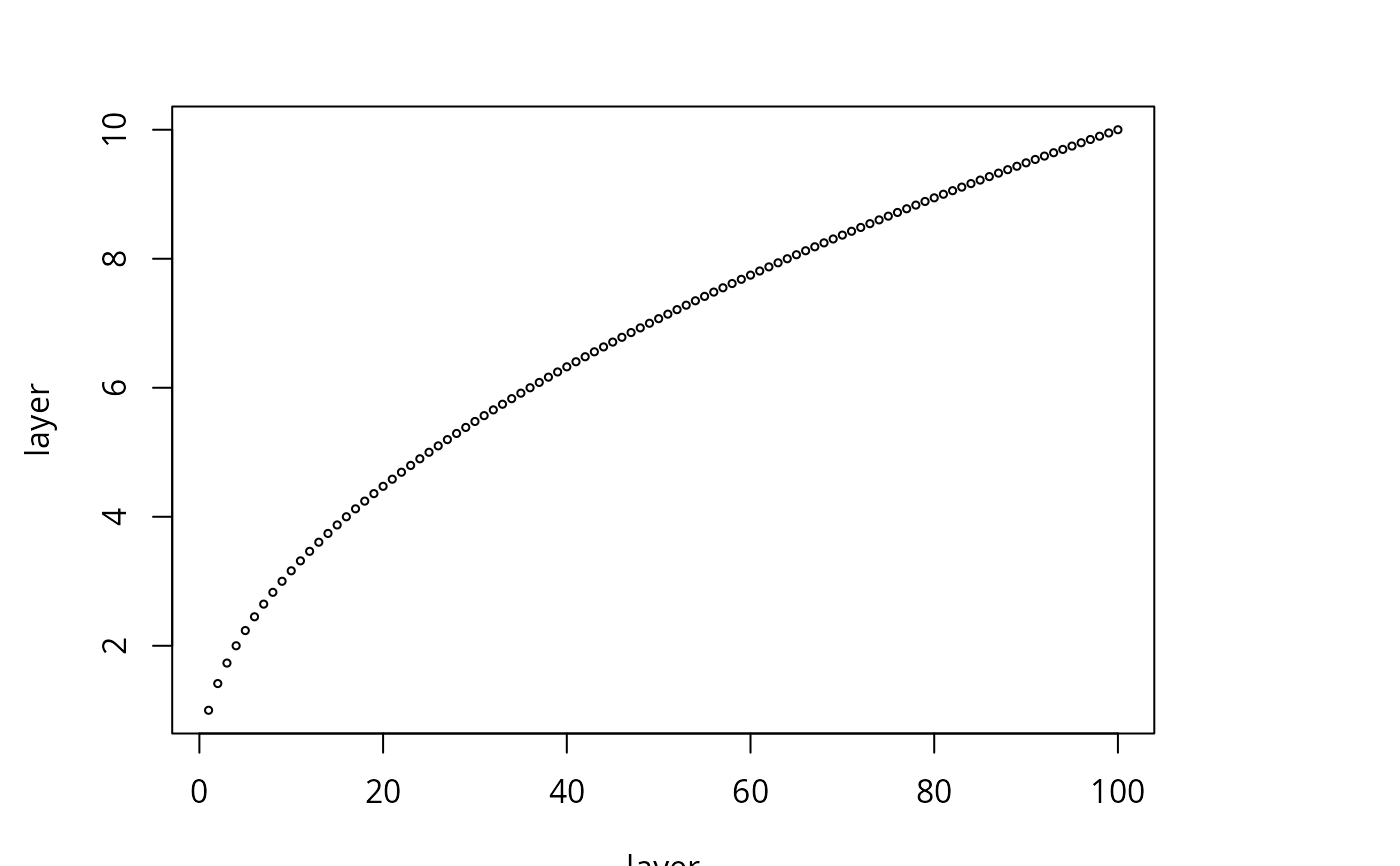
r2 <- sqrt(r)
plot(r, r2)
# Scatterplot of 2 RasterLayers
r2 <- sqrt(r)
plot(r, r2)
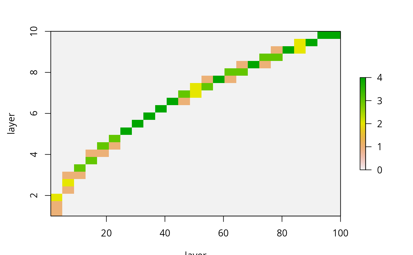
 plot(r, r2, gridded=TRUE)
 # Multi-layer object (RasterStack / Brick)
s <- stack(r, r2, r/r)
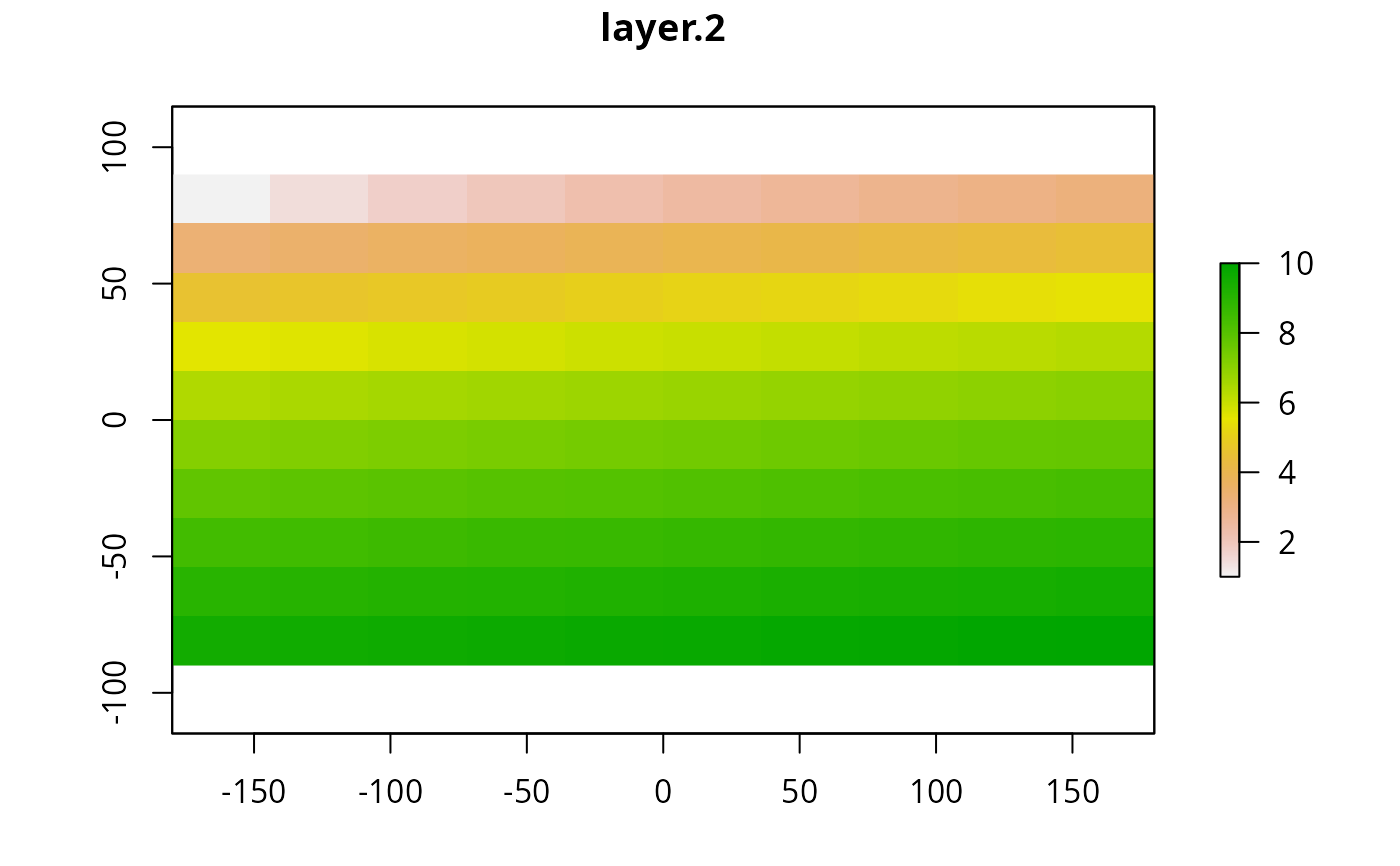
plot(s, 2)
# Multi-layer object (RasterStack / Brick)
s <- stack(r, r2, r/r)
plot(s, 2)
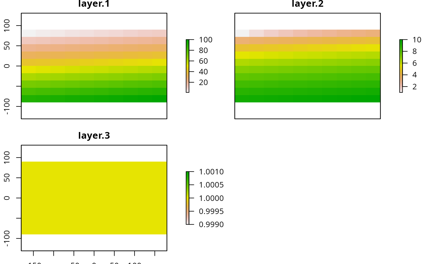
 plot(s)
 # two objects, different range, one scale:
values(r) <- runif(ncell(r))
r2 <- r/2
brks <- seq(0, 1, by=0.1)
nb <- length(brks)-1
cols <- rev(terrain.colors(nb))
par(mfrow=c(1,2))
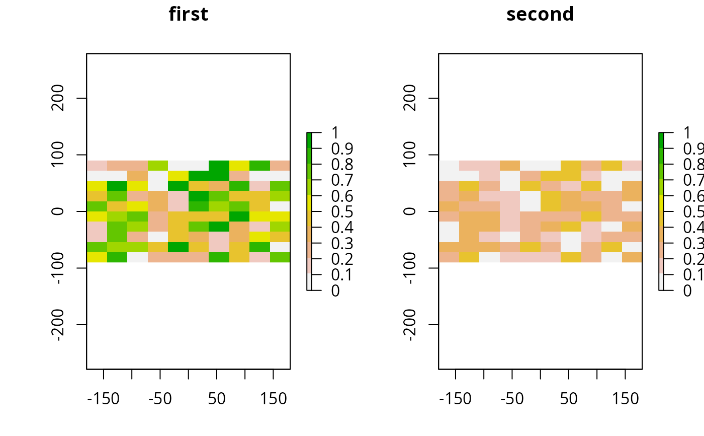
plot(r, breaks=brks, col=cols, lab.breaks=brks, zlim=c(0,1), main='first')
plot(r2, breaks=brks, col=cols, lab.breaks=brks, zlim=c(0,1), main='second')
# two objects, different range, one scale:
values(r) <- runif(ncell(r))
r2 <- r/2
brks <- seq(0, 1, by=0.1)
nb <- length(brks)-1
cols <- rev(terrain.colors(nb))
par(mfrow=c(1,2))
plot(r, breaks=brks, col=cols, lab.breaks=brks, zlim=c(0,1), main='first')
plot(r2, breaks=brks, col=cols, lab.breaks=brks, zlim=c(0,1), main='second')
 # breaks and labels
x <- raster(nc=10, nr=10)
values(x) <- runif(ncell(x))
brk <- c(0, 0.25, 0.75, 1)
arg <- list(at=c(0.12,0.5,0.87), labels=c("Low","Med.","High"))
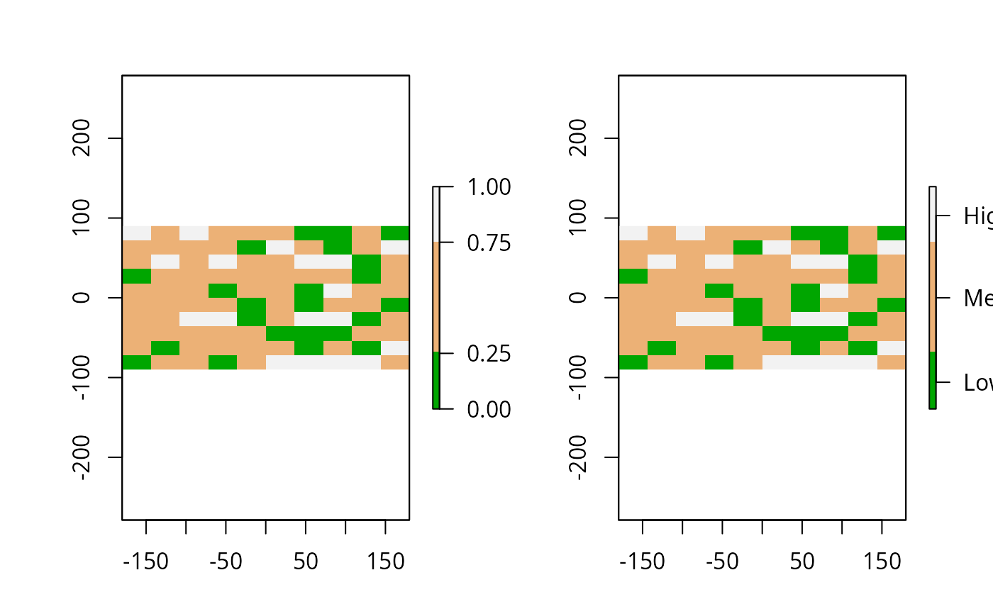
plot(x, col=terrain.colors(3), breaks=brk)
plot(x, col=terrain.colors(3), breaks=brk, axis.args=arg)
# breaks and labels
x <- raster(nc=10, nr=10)
values(x) <- runif(ncell(x))
brk <- c(0, 0.25, 0.75, 1)
arg <- list(at=c(0.12,0.5,0.87), labels=c("Low","Med.","High"))
plot(x, col=terrain.colors(3), breaks=brk)
plot(x, col=terrain.colors(3), breaks=brk, axis.args=arg)
 par(mfrow=c(1,1))
# color ramp
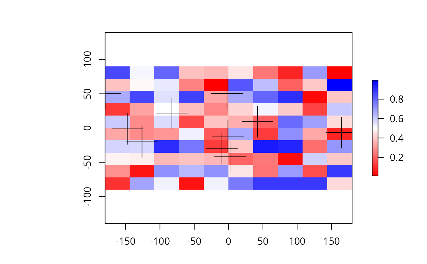
plot(x, col=colorRampPalette(c("red", "white", "blue"))(255))
# adding random points to the map
xy <- cbind(-180 + runif(10) * 360, -90 + runif(10) * 180)
points(xy, pch=3, cex=5)
par(mfrow=c(1,1))
# color ramp
plot(x, col=colorRampPalette(c("red", "white", "blue"))(255))
# adding random points to the map
xy <- cbind(-180 + runif(10) * 360, -90 + runif(10) * 180)
points(xy, pch=3, cex=5)
 # for SpatialPolygons do
# plot(pols, add=TRUE)
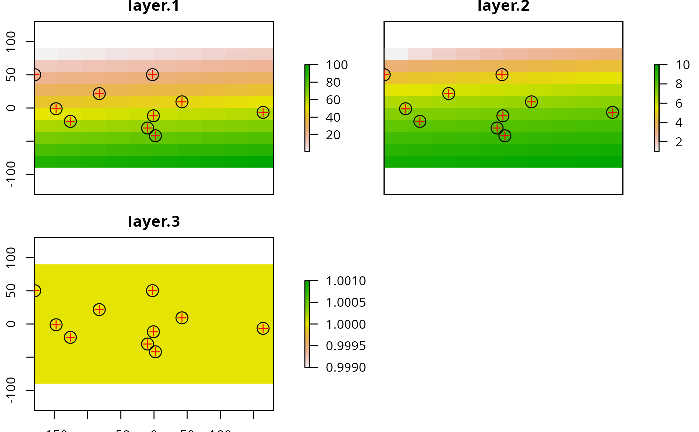
# adding the same points to each map of each layer of a RasterStack
fun <- function() {
points(xy, cex=2)
points(xy, pch=3, col='red')
}
plot(s, addfun=fun)
# for SpatialPolygons do
# plot(pols, add=TRUE)
# adding the same points to each map of each layer of a RasterStack
fun <- function() {
points(xy, cex=2)
points(xy, pch=3, col='red')
}
plot(s, addfun=fun)