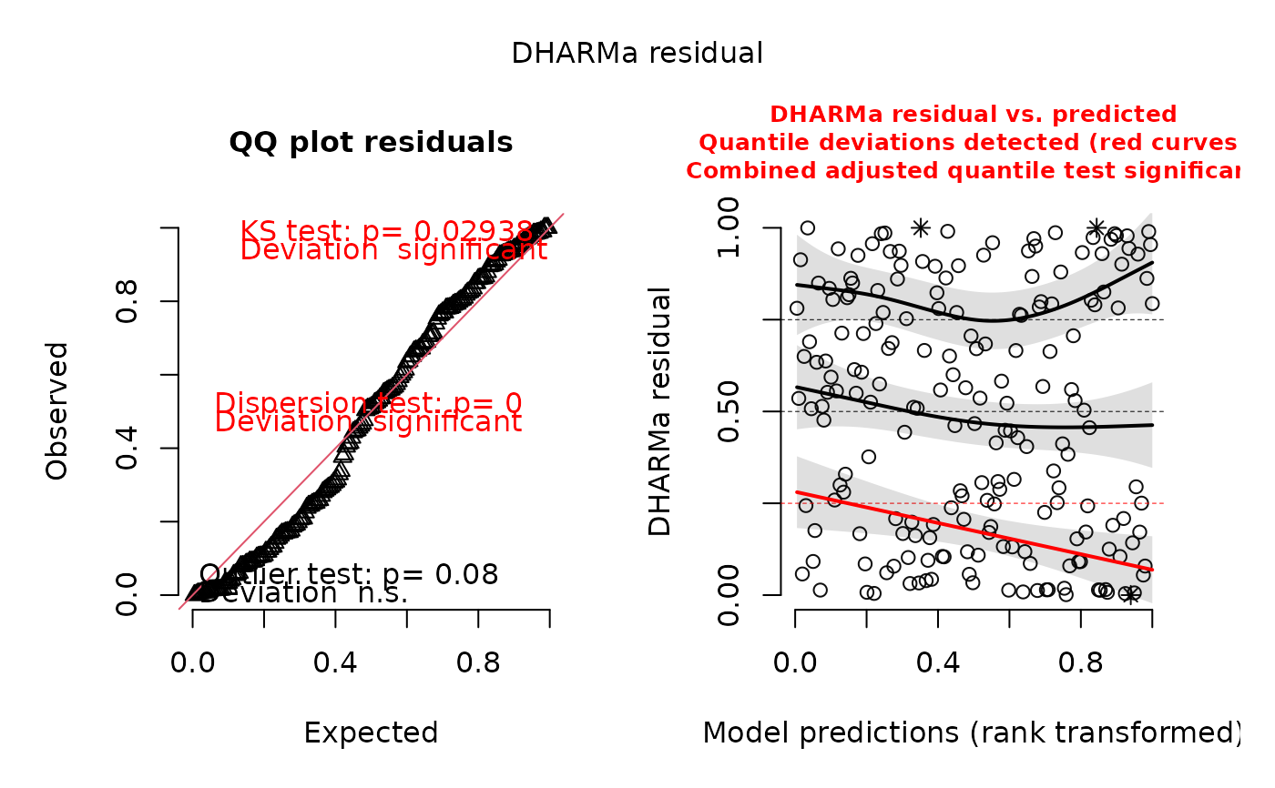
This S3 function creates standard plots for the simulated residuals contained in an object of class DHARMa, using plotQQunif (left panel) and plotResiduals (right panel).
Usage
# S3 method for class 'DHARMa'
plot(x, title = "DHARMa residual", ...)
Arguments
- x
an object of class DHARMa with simulated residuals created by simulateResiduals.
- title
the title for both panels (plotted via mtext, outer = TRUE).
- ...
further options for plotResiduals. Consider in particular parameters quantreg, rank and asFactor. xlab, ylab and main cannot be changed when using plot.DHARMa, but can be changed when using plotResiduals.
Details
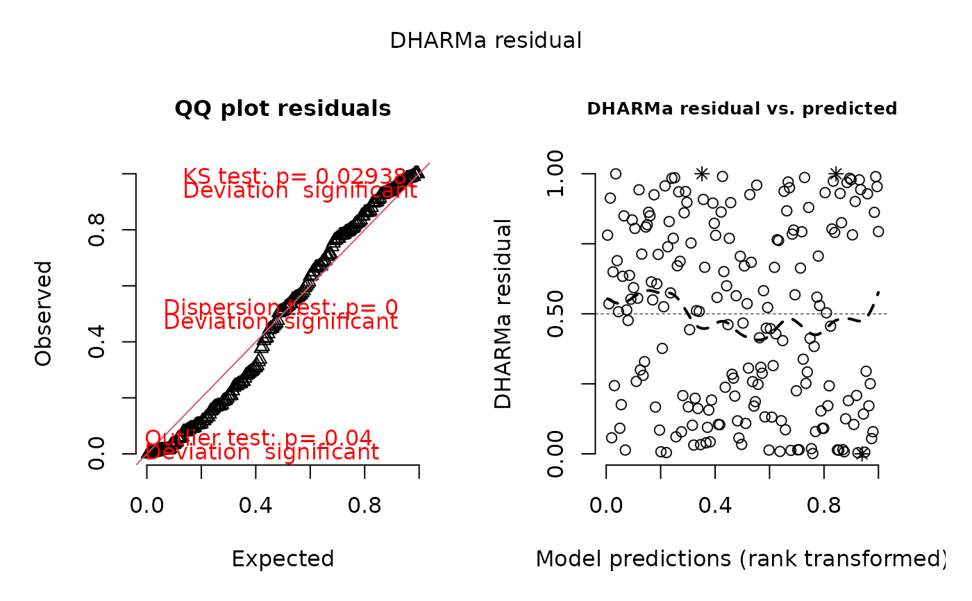
The function creates a plot with two panels. The left panel is a uniform qq plot (calling plotQQunif), and the right panel shows residuals against predicted values (calling plotResiduals), with outliers as a star/asterisk and highlighted in red if outlier test is significant (default color but see Note).
Very briefly, we would expect that a correctly specified model shows:
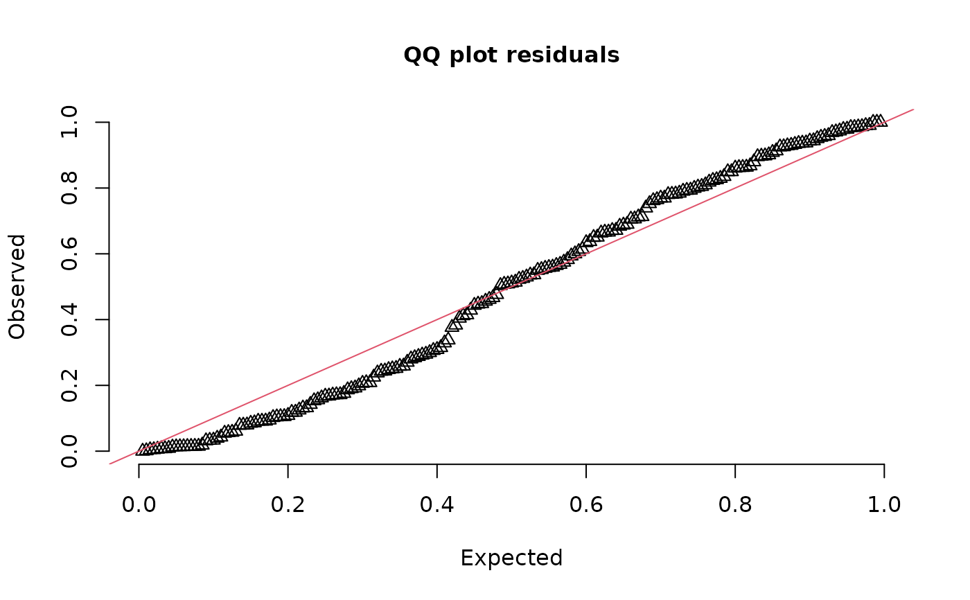
a) a straight 1-1 line, as well as non-significance of the displayed tests in the qq-plot (left) -> evidence for a correct overall residual distribution (for more details on the interpretation of this plot, see plotQQunif)
b) visual homogeneity of residuals in both vertical and horizontal direction, as well as non-significance of quantile tests in the res ~ predictor plot (for more details on the interpretation of this plot, see plotResiduals)
Deviations from these expectations can be interpreted similar to a linear regression. See the vignette for detailed examples.
Note that, unlike plotResiduals, plot.DHARMa command uses the default rank = T.
Note
The color for highlighting outliers and significant tests can be changed by setting options(DHARMaSignalColor = "red") to a different color. See getOption("DHARMaSignalColor") for the current setting. This is convenient for a color-blind friendly display, since red and black are difficult for some people to separate.
Examples
testData = createData(sampleSize = 200, family = poisson(),
fixedEffects = c(1,1),
randomEffectVariance = 1, numGroups = 10)
testData$Environment2[1] = NA
fittedModel <- glm(observedResponse ~ Environment1 + Environment2,
family = "poisson", data = testData)
simulationOutput <- simulateResiduals(fittedModel = fittedModel)
######### main plotting function #############
plot(simulationOutput)
 # for all functions, quantreg = T (default) will be more informative
# but slower. Alternative:
plot(simulationOutput, quantreg = FALSE)
# for all functions, quantreg = T (default) will be more informative
# but slower. Alternative:
plot(simulationOutput, quantreg = FALSE)
 ############# Distribution ######################
plotQQunif(simulationOutput = simulationOutput,
testDispersion = FALSE,
testUniformity = FALSE,
testOutliers = FALSE)
############# Distribution ######################
plotQQunif(simulationOutput = simulationOutput,
testDispersion = FALSE,
testUniformity = FALSE,
testOutliers = FALSE)
 hist(simulationOutput)