Generic res ~ pred scatter plot with spline or quantile regression on top

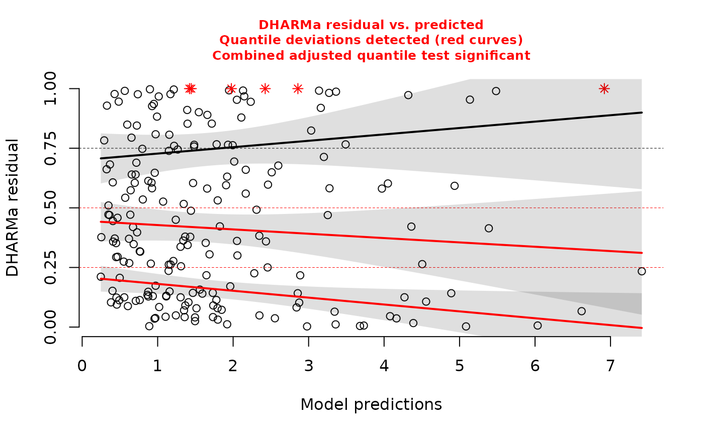
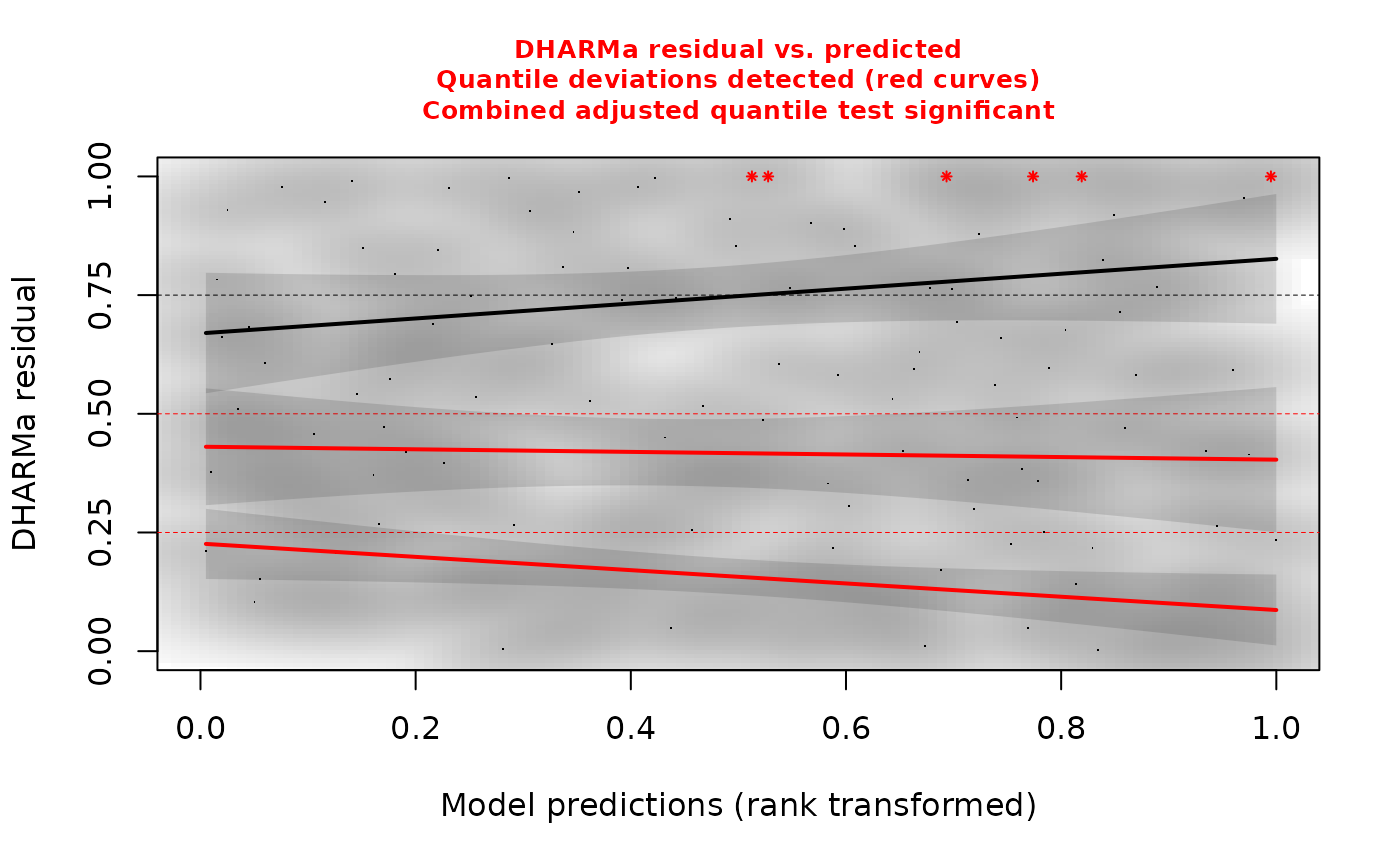
The function creates a generic residual plot with either spline or quantile regression to highlight patterns in the residuals. Outliers are marked in star/asterisk form and highlighted in red if the outlier test is significant.

Usage

plotResiduals(simulationOutput, form = NULL, quantreg = NULL,
  rank = TRUE, asFactor = NULL, smoothScatter = NULL,
  quantiles = c(0.25, 0.5, 0.75), absoluteDeviation = FALSE, ...)

Arguments

simulationOutput: an object, usually a DHARMa object, from which residual values can be extracted. Alternatively, a vector with residuals or a fitted model can be provided, which will then be transformed into a DHARMa object.
form: optional predictor(s) against which the residuals should be plotted. Default is to use the predicted(simulationOutput). Recommended to specify as formula. Use form = ~. to plot against all predictors. See details.
quantreg: whether to perform a quantile regression based on testQuantiles or a smooth spline around the mean. Default NULL chooses T for nObs < 10000, and F otherwise.
rank: if T, the values provided in form will be rank transformed. This will usually make patterns easier to spot visually, especially if the distribution of the predictor is skewed. If form is a factor, this has no effect.
asFactor: should a numeric predictor provided in form be treated as a factor. Default is to choose this for < 10 unique values, as long as enough predictions are available to draw a boxplot.
smoothScatter: if T, a smooth scatter plot will plotted instead of a normal scatter plot. This makes sense when the number of residuals is very large. Default NULL chooses T for nObs > 10000, and F otherwise.
quantiles: for a quantile regression, which quantiles should be plotted. Default is 0.25, 0.5, 0.75.
absoluteDeviation: if T, switch from displaying normal quantile residuals to absolute deviation from the mean expectation of 0.5 (calculated as 2 * abs(res - 0.5)). The purpose of this is to test explicitly for heteroskedasticity, see details.
...: additional arguments to plot / boxplot.

Value

If quantile tests are performed, the function returns them invisibly.

Details

The function plots residuals against a predictor (by default against the fitted value, extracted from the DHARMa object, or any other predictor). The shaded gray areas indicate 95% confidence intervals of the quantile estimates (1.96 * standard error).

Outliers are drawn if simulationOutput is a DHARMa object and highlighted in red if the outlier test is significant (for information on definition and interpretation of outliers, see testOutliers). See the note below to change the highlighting color of the outliers.

To provide a visual aid for detecting deviations from uniformity in the y-direction, the plot function calculates an (optional) quantile regression of the residuals, by default for the 0.25, 0.5 and 0.75 quantiles. Since the residuals should be uniformly distributed for a correctly specified model, the theoretical expectations for these regressions are straight lines at 0.25, 0.5 and 0.75, shown as dashed black lines on the plot. However, even for a perfect model, some deviation from these expectations is to be expected by chance, especially if the sample size is small. The function therefore tests whether the deviation of the fitted quantile regression from the expectation is significant, using testQuantiles. If so, the significant quantile regression is highlighted in red (as default) and a warning is displayed in the plot. See the note below to change the color of significant quantile lines.

Overdispersion typically manifests itself as Q1 (0.25) deviating towards 0 and Q3 (0.75) deviating towards 1. Heteroskedasticity manifests itself as non-parallel quantile lines. To diagnose heteroskedasticity and overdispersion, it can be helpful to additionally plot the absolute deviation of the residuals from the mean expectation of 0.5, using the option absoluteDeviation = T. In this case, we would again expect Q1-Q3 quantile lines at 0.25, 0.5, 0.75, but greater dispersion (also locally in the case of heteroskedasticity) always manifests itself in deviations towards 1.

The quantile regression can take some time to calculate, especially for larger datasets. For this reason, quantreg = F can be set to generate a smooth spline instead. This is the default for n > 10000.

If form is specified as a formula, e.g. form = ~ your_predictor, NAs will be handled automatically (recommended). If form = ~., separate plots for all predictors in the model are produced. If form = ~ predictor1 + predictor2, a separate plot for each specified predictor is produced. If an additional grouping variable is specified, e.g. form = ~ predictor|group, a separate plot for the predictor within each grouping level is produced. Be careful with this command: if you have many levels, the plot may not display nicely. If you are interested in a specific group, you can use form = ~ predictor|group == "group_level". If form is not a formula, e.g. form = data$predictor, NAs are not handled automatically. For phyr and gamm4$mer models, you need to specify form in this way.

If the predictor is a factor, a boxplot will be plotted instead of a scatter plot. The distribution for each factor level should be uniformly distributed, so the box should go from 0.25 to 0.75, with the median line at 0.5 (within-group). To test if deviations from those expectations are significant, KS-tests per group and a Levene test for homogeneity of variances are performed. See testCategorical for details.

Note

If nObs > 10,000, the scatter plot is replaced by graphics::smoothScatter().

The color for highlighting outliers and quantile lines/splines with significant tests can be changed by setting options(DHARMaSignalColor = "red") to a different color. See getOption("DHARMaSignalColor") for the current setting. This is convenient for a color-blind friendly display, since red and black are difficult for some people to distinguish.

Examples

testData = createData(sampleSize = 200, family = poisson(),
                      fixedEffects = c(1,1),
                      randomEffectVariance = 1, numGroups = 10)
testData$Environment2[1] = NA
fittedModel <- glm(observedResponse ~ Environment1 + Environment2,
                   family = "poisson", data = testData)
simulationOutput <- simulateResiduals(fittedModel = fittedModel)

#############  residual plots  ###############

# Default in DHARMa is to show predictions rank transformed
# if you want plots based on raw predictions, use rank = F
plotResiduals(simulationOutput, rank = FALSE)


# smooth scatter plot - default for large datasets with n > 10,000
plotResiduals(simulationOutput, rank = TRUE, smoothScatter = TRUE)


if (FALSE) { # \dontrun{

  # It is very advisable to plot the residual against all predictors
  # the following syntax uses the predictor values from the fitted model
  plotResiduals(simulationOutput, form = ~ Environment1)

  # plot against all predictors
  plotResiduals(simulationOutput, form = ~.)

  # if pred is a factor, or if asFactor = TRUE, will produce a boxplot
  plotResiduals(simulationOutput, form = ~group)

  # plot residuals against multiple predictors at once
  plotResiduals(simulationOutput, form = ~Environment1 + Environment2)

  # plot residuals against a predictor for all respective group levels
  plotResiduals(simulationOutput, form = ~Environment1|group)

  # plot residuals against a predictor for a specific group level, here group 1
  plotResiduals(simulationOutput, form = ~Environment1|group == "1")


  # alternatively, you can plot against a variable from the global environment
  # in this case, the model function automatically removed one row of observations
  # because there was an NA in Environment2. When using the variable Environment1
  # from the global environment, we have to remove this observation as well
  plotResiduals(simulationOutput,
                form = testData$Environment1[complete.cases(testData)])


  # to diagnose overdispersion and heteroskedasticity it can be useful to
  # display residuals as absolute deviation from the expected mean 0.5
  plotResiduals(simulationOutput, absoluteDeviation = TRUE)

  # All these options can also be provided to the main plotting function

  # If you want to plot summaries per group, use recalculateResiduals
  # for details see help of recalculateResiduals
} # }