This function fits quantile regressions on the residuals, and compares their location to the expected location.
Usage
testQuantiles(simulationOutput, predictor = NULL, rank = TRUE,
  quantiles = c(0.25, 0.5, 0.75), plot = TRUE)
Arguments
- simulationOutput
an object of class DHARMa, either created via simulateResiduals for supported models or by createDHARMa for simulations created outside DHARMa, or a supported model. Providing a supported model directly is discouraged, because simulation settings cannot be changed in this case.
- predictor
an optional predictor variable to be used, instead of the predicted response (default). See details.
- rank
if TRUE, the values provided in predictor will be rank transformed. This will usually make patterns easier to spot visually, especially if the distribution of the predictor is skewed. If form is a factor, this has no effect.
- quantiles
the quantiles to be tested.
- plot
if TRUE, the function will create an additional plot.
Details
The function fits quantile regressions (via package qgam) on the residuals, and compares their location to the expected location (because of the uniform distribution, the expected location is 0.5 for the 0.5 quantile).
A significant p-value for the splines means the fitted spline deviates from a flat line at the expected location.
The p-values of the intercept and splines are combined into a total p-value via Benjamini & Hochberg adjustment to control the FDR.
Predictor can be a formula (e.g. predictor = ~predictor), in which case NAs are handled automatically (recommended). Predictor can also be a variable in your environment (e.g. predictor = data$predictor), but then you need to remove rows that were excluded by the model due to NAs by hand. For more details and a more flexible syntax for predictors, see the help of the argument form in plotResiduals.
When plotting (plot = TRUE), the shaded gray areas indicate 95% confidence intervals of the quantile estimates (1.96 * standard error).
Examples
testData = createData(sampleSize = 200, overdispersion = 0.0, randomEffectVariance = 0)
fittedModel <- glm(observedResponse ~ Environment1, family = "poisson", data = testData)
simulationOutput <- simulateResiduals(fittedModel = fittedModel)
# run the quantile test
x = testQuantiles(simulationOutput)
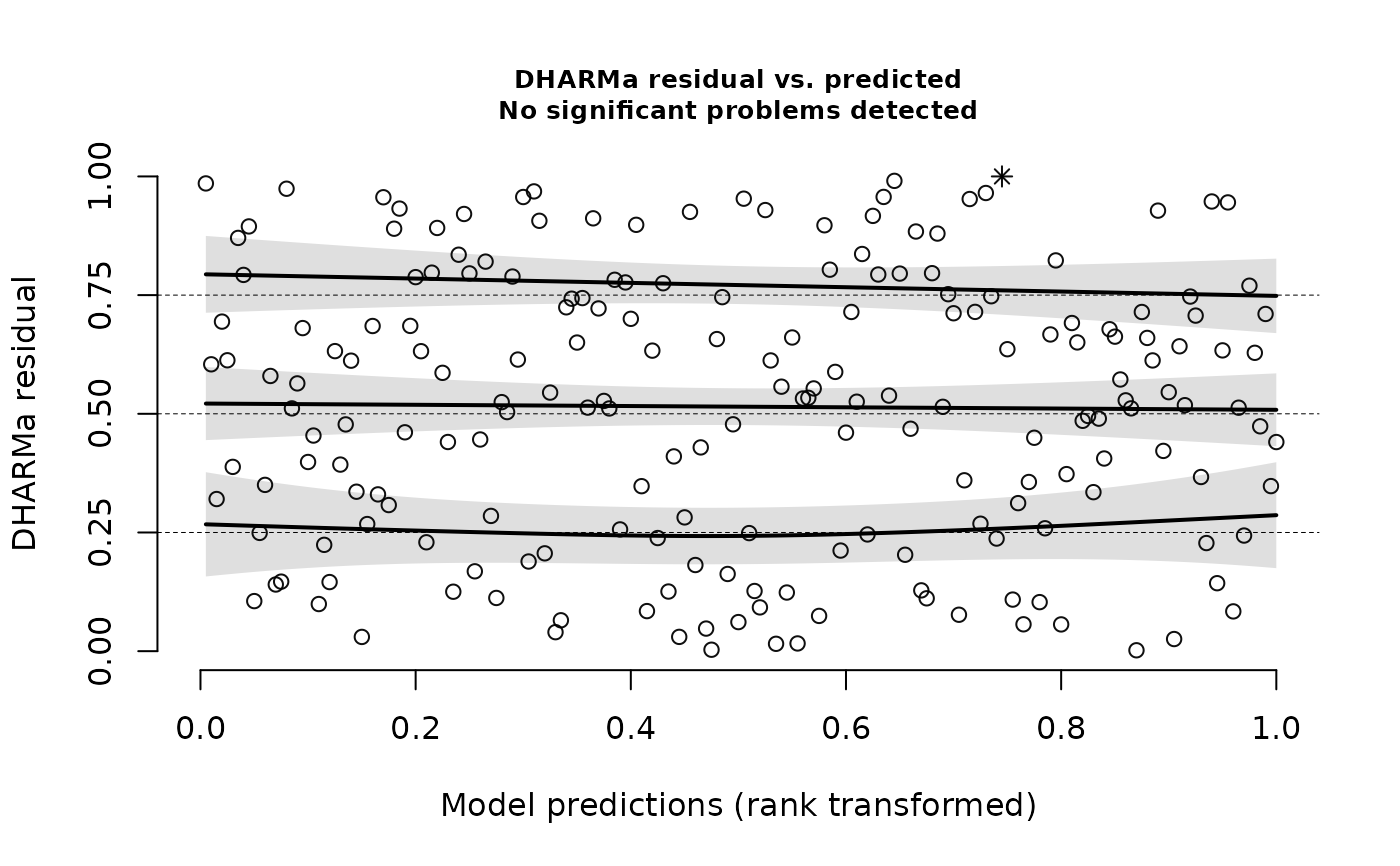 x # the test shows a combined p-value, corrected for multiple testing
#>
#> Test for location of quantiles via qgam
#>
#> data: res
#> p-value = 0.8462
#> alternative hypothesis: both
#>
if (FALSE) { # \dontrun{
# accessing results of the test
x$pvals # pvalues for the individual quantiles
x$qgamFits # access the fitted quantile regression
summary(x$qgamFits[[1]]) # summary of the first fitted quantile
# possible to test user-defined quantiles
testQuantiles(simulationOutput, quantiles = c(0.7))
# example with missing environmental predictor
fittedModel <- glm(observedResponse ~ 1 , family = "poisson", data = testData)
simulationOutput <- simulateResiduals(fittedModel = fittedModel)
# specified as formula (recommended)
testQuantiles(simulationOutput, predictor = ~Environment1)
# or as variable in your environment
testQuantiles(simulationOutput, predictor = testData$Environment1)
plot(simulationOutput)
plotResiduals(simulationOutput)
} # }
x # the test shows a combined p-value, corrected for multiple testing
#>
#> Test for location of quantiles via qgam
#>
#> data: res
#> p-value = 0.8462
#> alternative hypothesis: both
#>
if (FALSE) { # \dontrun{
# accessing results of the test
x$pvals # pvalues for the individual quantiles
x$qgamFits # access the fitted quantile regression
summary(x$qgamFits[[1]]) # summary of the first fitted quantile
# possible to test user-defined quantiles
testQuantiles(simulationOutput, quantiles = c(0.7))
# example with missing environmental predictor
fittedModel <- glm(observedResponse ~ 1 , family = "poisson", data = testData)
simulationOutput <- simulateResiduals(fittedModel = fittedModel)
# specified as formula (recommended)
testQuantiles(simulationOutput, predictor = ~Environment1)
# or as variable in your environment
testQuantiles(simulationOutput, predictor = testData$Environment1)
plot(simulationOutput)
plotResiduals(simulationOutput)
} # }