This function tests the overall uniformity of the simulated residuals in a DHARMa object.
Usage
testUniformity(simulationOutput, alternative = c("two.sided", "less",
  "greater"), plot = TRUE)
Arguments
- simulationOutput
an object of class DHARMa, either created via simulateResiduals for supported models or by createDHARMa for simulations created outside DHARMa, or a supported model. Providing a supported model directly is discouraged, because simulation settings cannot be changed in this case.
- alternative
a character string specifying whether the test should test if observations are "greater", "less" or "two.sided" compared to the simulated null hypothesis. See stats::ks.test for details.
- plot
if TRUE, plots calls plotQQunif as well.
Details
The function applies a stats::ks.test for uniformity on the simulated residuals.
Examples
testData = createData(sampleSize = 100, overdispersion = 0.5, randomEffectVariance = 0)
fittedModel <- glm(observedResponse ~ Environment1 , family = "poisson", data = testData)
simulationOutput <- simulateResiduals(fittedModel = fittedModel)
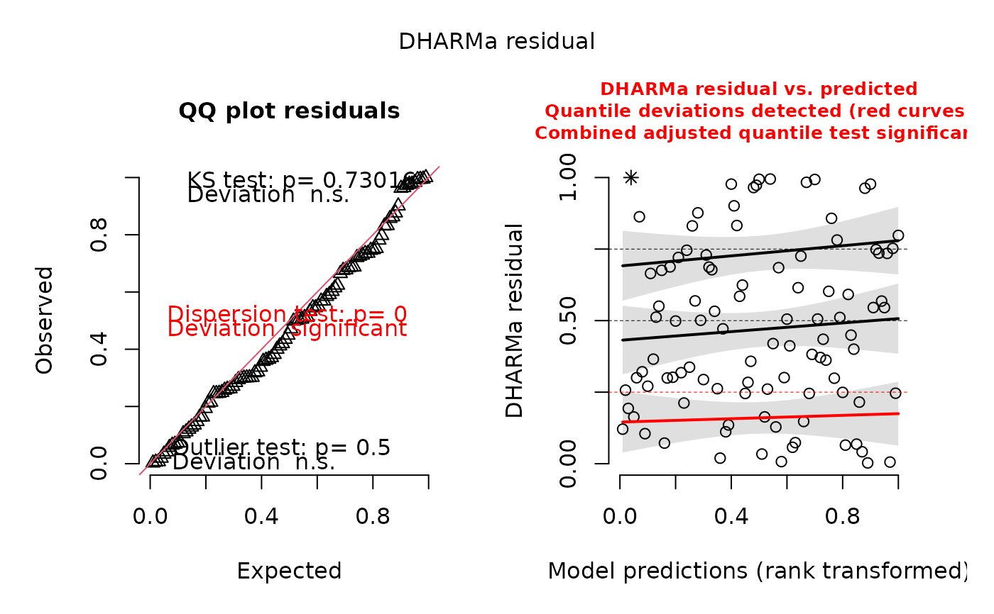
# the plot function shows 2 plots and runs 4 tests
# i) KS test i) Dispersion test iii) Outlier test iv) quantile test
plot(simulationOutput, quantreg = TRUE)
 # testResiduals tests distribution, dispersion and outliers
testResiduals(simulationOutput)
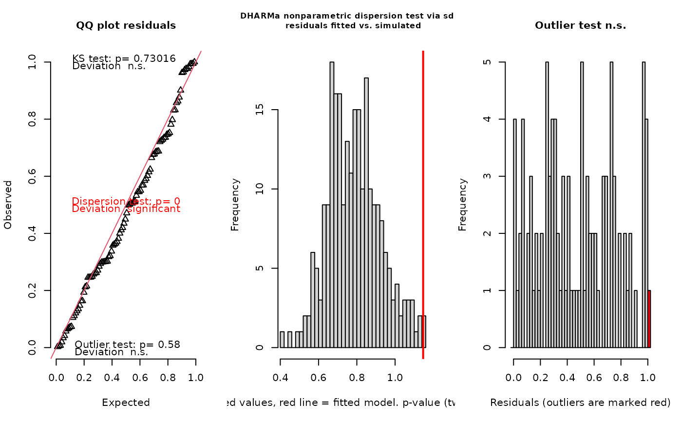
# testResiduals tests distribution, dispersion and outliers
testResiduals(simulationOutput)
 #> $uniformity
#>
#> Asymptotic one-sample Kolmogorov-Smirnov test
#>
#> data: simulationOutput$scaledResiduals
#> D = 0.068857, p-value = 0.7302
#> alternative hypothesis: two-sided
#>
#>
#> $dispersion
#>
#> DHARMa nonparametric dispersion test via sd of residuals fitted vs.
#> simulated
#>
#> data: simulationOutput
#> dispersion = 1.4559, p-value < 2.2e-16
#> alternative hypothesis: two.sided
#>
#>
#> $outliers
#>
#> DHARMa bootstrapped outlier test
#>
#> data: simulationOutput
#> outliers at both margin(s) = 1, observations = 100, p-value = 0.48
#> alternative hypothesis: two.sided
#> percent confidence interval:
#> 0.00 0.02
#> sample estimates:
#> outlier frequency (expected: 0.0029 )
#> 0.01
#>
#>
####### Individual tests #######
# KS test for correct distribution of residuals
testUniformity(simulationOutput)
#> $uniformity
#>
#> Asymptotic one-sample Kolmogorov-Smirnov test
#>
#> data: simulationOutput$scaledResiduals
#> D = 0.068857, p-value = 0.7302
#> alternative hypothesis: two-sided
#>
#>
#> $dispersion
#>
#> DHARMa nonparametric dispersion test via sd of residuals fitted vs.
#> simulated
#>
#> data: simulationOutput
#> dispersion = 1.4559, p-value < 2.2e-16
#> alternative hypothesis: two.sided
#>
#>
#> $outliers
#>
#> DHARMa bootstrapped outlier test
#>
#> data: simulationOutput
#> outliers at both margin(s) = 1, observations = 100, p-value = 0.48
#> alternative hypothesis: two.sided
#> percent confidence interval:
#> 0.00 0.02
#> sample estimates:
#> outlier frequency (expected: 0.0029 )
#> 0.01
#>
#>
####### Individual tests #######
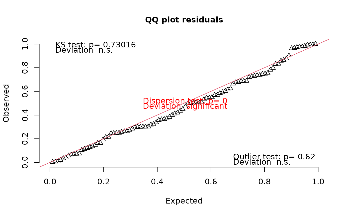
# KS test for correct distribution of residuals
testUniformity(simulationOutput)
 #>
#> Asymptotic one-sample Kolmogorov-Smirnov test
#>
#> data: simulationOutput$scaledResiduals
#> D = 0.068857, p-value = 0.7302
#> alternative hypothesis: two-sided
#>
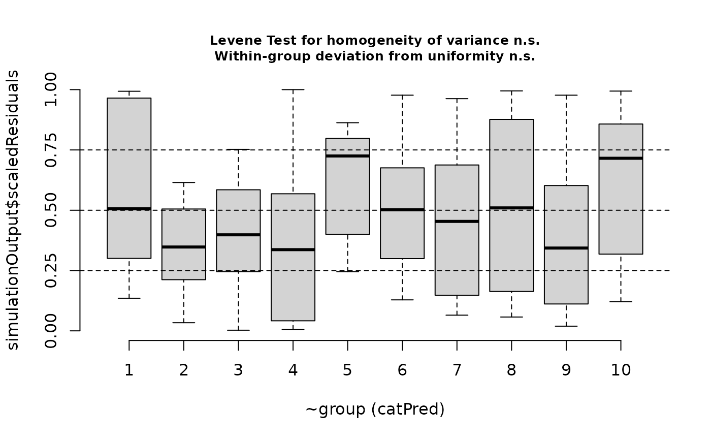
# KS test for correct distribution within and between groups
# group specified as formula (recommended)
testCategorical(simulationOutput, ~group)
#>
#> Asymptotic one-sample Kolmogorov-Smirnov test
#>
#> data: simulationOutput$scaledResiduals
#> D = 0.068857, p-value = 0.7302
#> alternative hypothesis: two-sided
#>
# KS test for correct distribution within and between groups
# group specified as formula (recommended)
testCategorical(simulationOutput, ~group)
 #> $uniformity
$details
#> catPred: 1
#>
#> Exact one-sample Kolmogorov-Smirnov test
#>
#> data: dd[x, ]
#> D = 0.26499, p-value = 0.4117
#> alternative hypothesis: two-sided
#>
#> ------------------------------------------------------------
#> catPred: 2
#>
#> Exact one-sample Kolmogorov-Smirnov test
#>
#> data: dd[x, ]
#> D = 0.38502, p-value = 0.07638
#> alternative hypothesis: two-sided
#>
#> ------------------------------------------------------------
#> catPred: 3
#>
#> Exact one-sample Kolmogorov-Smirnov test
#>
#> data: dd[x, ]
#> D = 0.27588, p-value = 0.3635
#> alternative hypothesis: two-sided
#>
#> ------------------------------------------------------------
#> catPred: 4
#>
#> Exact one-sample Kolmogorov-Smirnov test
#>
#> data: dd[x, ]
#> D = 0.33164, p-value = 0.1759
#> alternative hypothesis: two-sided
#>
#> ------------------------------------------------------------
#> catPred: 5
#>
#> Exact one-sample Kolmogorov-Smirnov test
#>
#> data: dd[x, ]
#> D = 0.32072, p-value = 0.2052
#> alternative hypothesis: two-sided
#>
#> ------------------------------------------------------------
#> catPred: 6
#>
#> Exact one-sample Kolmogorov-Smirnov test
#>
#> data: dd[x, ]
#> D = 0.21287, p-value = 0.681
#> alternative hypothesis: two-sided
#>
#> ------------------------------------------------------------
#> catPred: 7
#>
#> Exact one-sample Kolmogorov-Smirnov test
#>
#> data: dd[x, ]
#> D = 0.20682, p-value = 0.7132
#> alternative hypothesis: two-sided
#>
#> ------------------------------------------------------------
#> catPred: 8
#>
#> Exact one-sample Kolmogorov-Smirnov test
#>
#> data: dd[x, ]
#> D = 0.22539, p-value = 0.6134
#> alternative hypothesis: two-sided
#>
#> ------------------------------------------------------------
#> catPred: 9
#>
#> Exact one-sample Kolmogorov-Smirnov test
#>
#> data: dd[x, ]
#> D = 0.23467, p-value = 0.5636
#> alternative hypothesis: two-sided
#>
#> ------------------------------------------------------------
#> catPred: 10
#>
#> Exact one-sample Kolmogorov-Smirnov test
#>
#> data: dd[x, ]
#> D = 0.28507, p-value = 0.3258
#> alternative hypothesis: two-sided
#>
#>
#> $uniformity$p.value
#> [1] 0.41174486 0.07637943 0.36345412 0.17587683 0.20521280 0.68097859
#> [7] 0.71317472 0.61343756 0.56361305 0.32579853
#>
#> $uniformity$p.value.cor
#> [1] 1.0000000 0.7637943 1.0000000 1.0000000 1.0000000 1.0000000 1.0000000
#> [8] 1.0000000 1.0000000 1.0000000
#>
#>
#> $homogeneity
#> Levene's Test for Homogeneity of Variance (center = median)
#> Df F value Pr(>F)
#> group 9 1.338 0.2288
#> 90
#>
# group specified as variable in your environment
testCategorical(simulationOutput, testData$group)
#> $uniformity
#> $uniformity$details
#> catPred: 1
#>
#> Exact one-sample Kolmogorov-Smirnov test
#>
#> data: dd[x, ]
#> D = 0.26499, p-value = 0.4117
#> alternative hypothesis: two-sided
#>
#> ------------------------------------------------------------
#> catPred: 2
#>
#> Exact one-sample Kolmogorov-Smirnov test
#>
#> data: dd[x, ]
#> D = 0.38502, p-value = 0.07638
#> alternative hypothesis: two-sided
#>
#> ------------------------------------------------------------
#> catPred: 3
#>
#> Exact one-sample Kolmogorov-Smirnov test
#>
#> data: dd[x, ]
#> D = 0.27588, p-value = 0.3635
#> alternative hypothesis: two-sided
#>
#> ------------------------------------------------------------
#> catPred: 4
#>
#> Exact one-sample Kolmogorov-Smirnov test
#>
#> data: dd[x, ]
#> D = 0.33164, p-value = 0.1759
#> alternative hypothesis: two-sided
#>
#> ------------------------------------------------------------
#> catPred: 5
#>
#> Exact one-sample Kolmogorov-Smirnov test
#>
#> data: dd[x, ]
#> D = 0.32072, p-value = 0.2052
#> alternative hypothesis: two-sided
#>
#> ------------------------------------------------------------
#> catPred: 6
#>
#> Exact one-sample Kolmogorov-Smirnov test
#>
#> data: dd[x, ]
#> D = 0.21287, p-value = 0.681
#> alternative hypothesis: two-sided
#>
#> ------------------------------------------------------------
#> catPred: 7
#>
#> Exact one-sample Kolmogorov-Smirnov test
#>
#> data: dd[x, ]
#> D = 0.20682, p-value = 0.7132
#> alternative hypothesis: two-sided
#>
#> ------------------------------------------------------------
#> catPred: 8
#>
#> Exact one-sample Kolmogorov-Smirnov test
#>
#> data: dd[x, ]
#> D = 0.22539, p-value = 0.6134
#> alternative hypothesis: two-sided
#>
#> ------------------------------------------------------------
#> catPred: 9
#>
#> Exact one-sample Kolmogorov-Smirnov test
#>
#> data: dd[x, ]
#> D = 0.23467, p-value = 0.5636
#> alternative hypothesis: two-sided
#>
#> ------------------------------------------------------------
#> catPred: 10
#>
#> Exact one-sample Kolmogorov-Smirnov test
#>
#> data: dd[x, ]
#> D = 0.28507, p-value = 0.3258
#> alternative hypothesis: two-sided
#>
#>
#> $uniformity$p.value
#> [1] 0.41174486 0.07637943 0.36345412 0.17587683 0.20521280 0.68097859
#> [7] 0.71317472 0.61343756 0.56361305 0.32579853
#>
#> $uniformity$p.value.cor
#> [1] 1.0000000 0.7637943 1.0000000 1.0000000 1.0000000 1.0000000 1.0000000
#> [8] 1.0000000 1.0000000 1.0000000
#>
#>
#> $homogeneity
#> Levene's Test for Homogeneity of Variance (center = median)
#> Df F value Pr(>F)
#> group 9 1.338 0.2288
#> 90
#>
# group specified as variable in your environment
testCategorical(simulationOutput, testData$group)
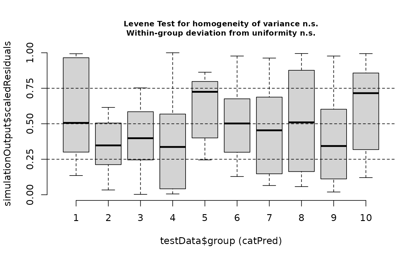 #> $uniformity
$details
#> catPred: 1
#>
#> Exact one-sample Kolmogorov-Smirnov test
#>
#> data: dd[x, ]
#> D = 0.26499, p-value = 0.4117
#> alternative hypothesis: two-sided
#>
#> ------------------------------------------------------------
#> catPred: 2
#>
#> Exact one-sample Kolmogorov-Smirnov test
#>
#> data: dd[x, ]
#> D = 0.38502, p-value = 0.07638
#> alternative hypothesis: two-sided
#>
#> ------------------------------------------------------------
#> catPred: 3
#>
#> Exact one-sample Kolmogorov-Smirnov test
#>
#> data: dd[x, ]
#> D = 0.27588, p-value = 0.3635
#> alternative hypothesis: two-sided
#>
#> ------------------------------------------------------------
#> catPred: 4
#>
#> Exact one-sample Kolmogorov-Smirnov test
#>
#> data: dd[x, ]
#> D = 0.33164, p-value = 0.1759
#> alternative hypothesis: two-sided
#>
#> ------------------------------------------------------------
#> catPred: 5
#>
#> Exact one-sample Kolmogorov-Smirnov test
#>
#> data: dd[x, ]
#> D = 0.32072, p-value = 0.2052
#> alternative hypothesis: two-sided
#>
#> ------------------------------------------------------------
#> catPred: 6
#>
#> Exact one-sample Kolmogorov-Smirnov test
#>
#> data: dd[x, ]
#> D = 0.21287, p-value = 0.681
#> alternative hypothesis: two-sided
#>
#> ------------------------------------------------------------
#> catPred: 7
#>
#> Exact one-sample Kolmogorov-Smirnov test
#>
#> data: dd[x, ]
#> D = 0.20682, p-value = 0.7132
#> alternative hypothesis: two-sided
#>
#> ------------------------------------------------------------
#> catPred: 8
#>
#> Exact one-sample Kolmogorov-Smirnov test
#>
#> data: dd[x, ]
#> D = 0.22539, p-value = 0.6134
#> alternative hypothesis: two-sided
#>
#> ------------------------------------------------------------
#> catPred: 9
#>
#> Exact one-sample Kolmogorov-Smirnov test
#>
#> data: dd[x, ]
#> D = 0.23467, p-value = 0.5636
#> alternative hypothesis: two-sided
#>
#> ------------------------------------------------------------
#> catPred: 10
#>
#> Exact one-sample Kolmogorov-Smirnov test
#>
#> data: dd[x, ]
#> D = 0.28507, p-value = 0.3258
#> alternative hypothesis: two-sided
#>
#>
#> $uniformity$p.value
#> [1] 0.41174486 0.07637943 0.36345412 0.17587683 0.20521280 0.68097859
#> [7] 0.71317472 0.61343756 0.56361305 0.32579853
#>
#> $uniformity$p.value.cor
#> [1] 1.0000000 0.7637943 1.0000000 1.0000000 1.0000000 1.0000000 1.0000000
#> [8] 1.0000000 1.0000000 1.0000000
#>
#>
#> $homogeneity
#> Levene's Test for Homogeneity of Variance (center = median)
#> Df F value Pr(>F)
#> group 9 1.338 0.2288
#> 90
#>
# Dispersion test - for details see ?testDispersion
testDispersion(simulationOutput) # tests under and overdispersion
#> $uniformity
#> $uniformity$details
#> catPred: 1
#>
#> Exact one-sample Kolmogorov-Smirnov test
#>
#> data: dd[x, ]
#> D = 0.26499, p-value = 0.4117
#> alternative hypothesis: two-sided
#>
#> ------------------------------------------------------------
#> catPred: 2
#>
#> Exact one-sample Kolmogorov-Smirnov test
#>
#> data: dd[x, ]
#> D = 0.38502, p-value = 0.07638
#> alternative hypothesis: two-sided
#>
#> ------------------------------------------------------------
#> catPred: 3
#>
#> Exact one-sample Kolmogorov-Smirnov test
#>
#> data: dd[x, ]
#> D = 0.27588, p-value = 0.3635
#> alternative hypothesis: two-sided
#>
#> ------------------------------------------------------------
#> catPred: 4
#>
#> Exact one-sample Kolmogorov-Smirnov test
#>
#> data: dd[x, ]
#> D = 0.33164, p-value = 0.1759
#> alternative hypothesis: two-sided
#>
#> ------------------------------------------------------------
#> catPred: 5
#>
#> Exact one-sample Kolmogorov-Smirnov test
#>
#> data: dd[x, ]
#> D = 0.32072, p-value = 0.2052
#> alternative hypothesis: two-sided
#>
#> ------------------------------------------------------------
#> catPred: 6
#>
#> Exact one-sample Kolmogorov-Smirnov test
#>
#> data: dd[x, ]
#> D = 0.21287, p-value = 0.681
#> alternative hypothesis: two-sided
#>
#> ------------------------------------------------------------
#> catPred: 7
#>
#> Exact one-sample Kolmogorov-Smirnov test
#>
#> data: dd[x, ]
#> D = 0.20682, p-value = 0.7132
#> alternative hypothesis: two-sided
#>
#> ------------------------------------------------------------
#> catPred: 8
#>
#> Exact one-sample Kolmogorov-Smirnov test
#>
#> data: dd[x, ]
#> D = 0.22539, p-value = 0.6134
#> alternative hypothesis: two-sided
#>
#> ------------------------------------------------------------
#> catPred: 9
#>
#> Exact one-sample Kolmogorov-Smirnov test
#>
#> data: dd[x, ]
#> D = 0.23467, p-value = 0.5636
#> alternative hypothesis: two-sided
#>
#> ------------------------------------------------------------
#> catPred: 10
#>
#> Exact one-sample Kolmogorov-Smirnov test
#>
#> data: dd[x, ]
#> D = 0.28507, p-value = 0.3258
#> alternative hypothesis: two-sided
#>
#>
#> $uniformity$p.value
#> [1] 0.41174486 0.07637943 0.36345412 0.17587683 0.20521280 0.68097859
#> [7] 0.71317472 0.61343756 0.56361305 0.32579853
#>
#> $uniformity$p.value.cor
#> [1] 1.0000000 0.7637943 1.0000000 1.0000000 1.0000000 1.0000000 1.0000000
#> [8] 1.0000000 1.0000000 1.0000000
#>
#>
#> $homogeneity
#> Levene's Test for Homogeneity of Variance (center = median)
#> Df F value Pr(>F)
#> group 9 1.338 0.2288
#> 90
#>
# Dispersion test - for details see ?testDispersion
testDispersion(simulationOutput) # tests under and overdispersion
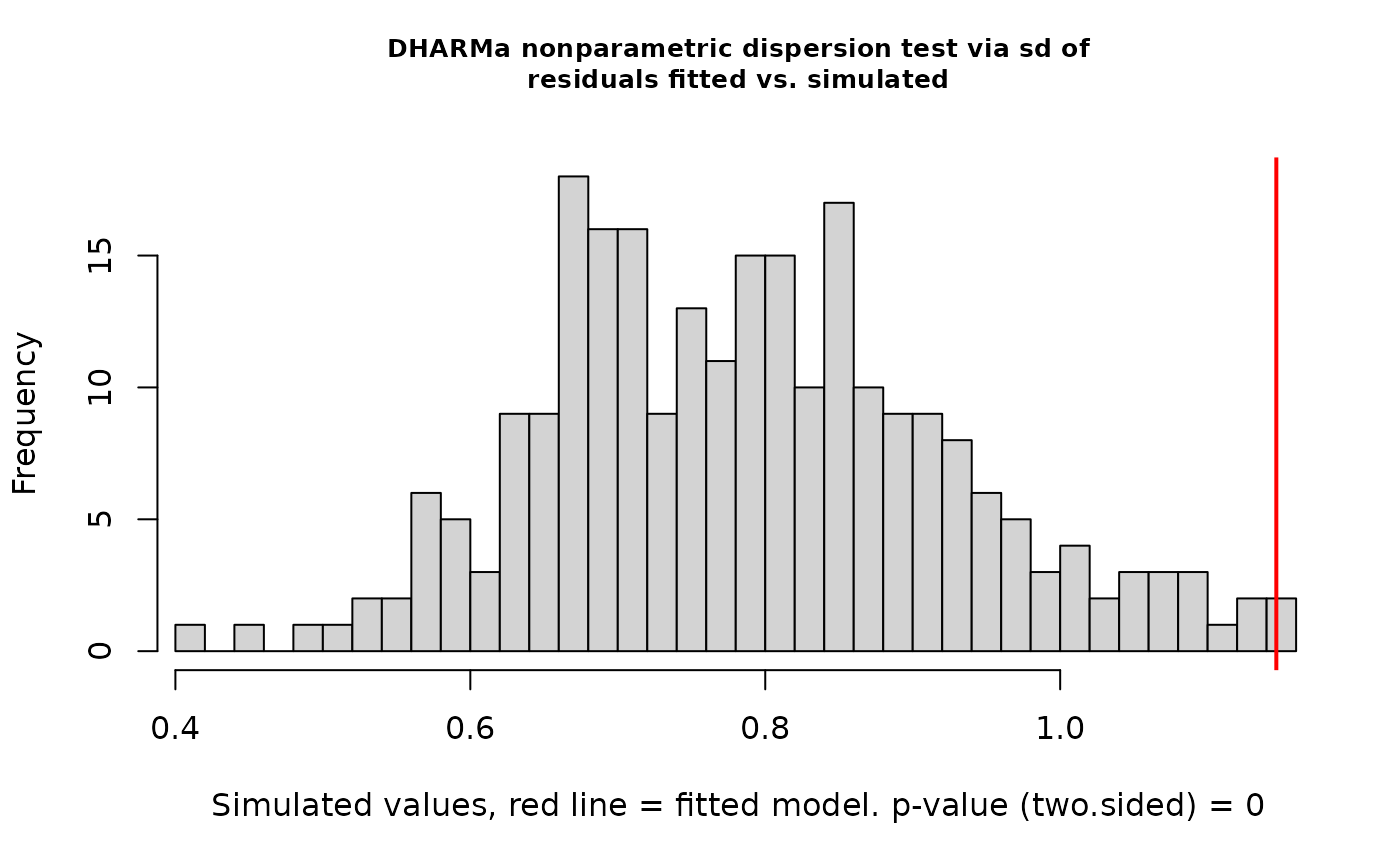 #>
#> DHARMa nonparametric dispersion test via sd of residuals fitted vs.
#> simulated
#>
#> data: simulationOutput
#> dispersion = 1.4559, p-value < 2.2e-16
#> alternative hypothesis: two.sided
#>
# Outlier test (number of observations outside simulation envelope)
# Use type = "boostrap" for exact values, see ?testOutliers
testOutliers(simulationOutput, type = "binomial")
#>
#> DHARMa nonparametric dispersion test via sd of residuals fitted vs.
#> simulated
#>
#> data: simulationOutput
#> dispersion = 1.4559, p-value < 2.2e-16
#> alternative hypothesis: two.sided
#>
# Outlier test (number of observations outside simulation envelope)
# Use type = "boostrap" for exact values, see ?testOutliers
testOutliers(simulationOutput, type = "binomial")
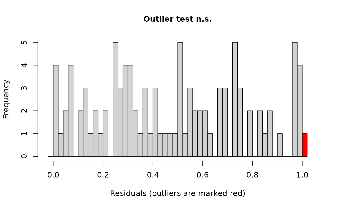 #>
#> DHARMa outlier test based on exact binomial test with approximate
#> expectations
#>
#> data: simulationOutput
#> outliers at both margin(s) = 2, observations = 100, p-value = 0.1898
#> alternative hypothesis: true probability of success is not equal to 0.007968127
#> 95 percent confidence interval:
#> 0.002431337 0.070383932
#> sample estimates:
#> frequency of outliers (expected: 0.00796812749003984 )
#> 0.02
#>
# testing zero inflation
testZeroInflation(simulationOutput)
#>
#> DHARMa outlier test based on exact binomial test with approximate
#> expectations
#>
#> data: simulationOutput
#> outliers at both margin(s) = 2, observations = 100, p-value = 0.1898
#> alternative hypothesis: true probability of success is not equal to 0.007968127
#> 95 percent confidence interval:
#> 0.002431337 0.070383932
#> sample estimates:
#> frequency of outliers (expected: 0.00796812749003984 )
#> 0.02
#>
# testing zero inflation
testZeroInflation(simulationOutput)
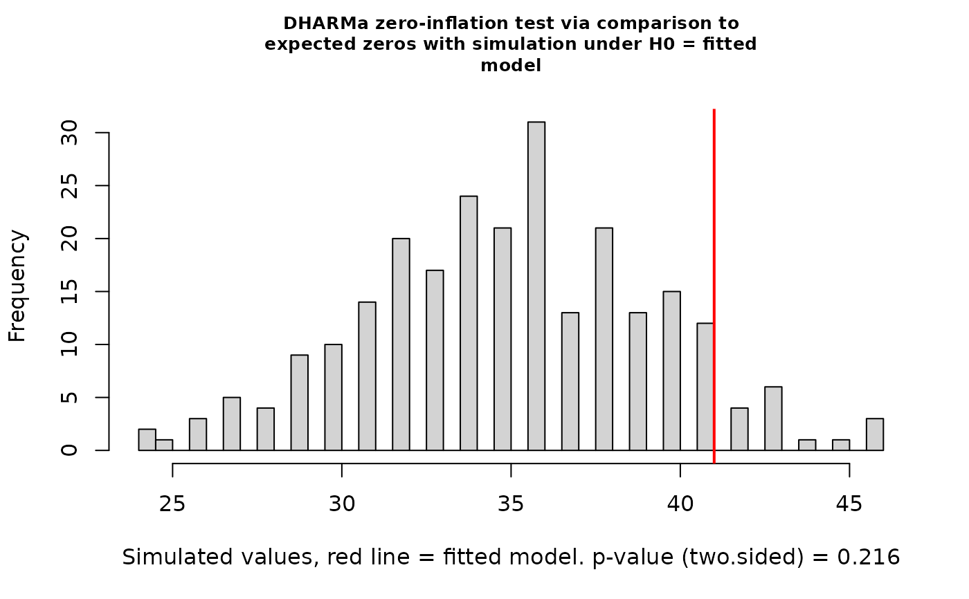 #>
#> DHARMa zero-inflation test via comparison to expected zeros with
#> simulation under H0 = fitted model
#>
#> data: simulationOutput
#> ratioObsSim = 1.1658, p-value = 0.216
#> alternative hypothesis: two.sided
#>
# testing generic summaries
countOnes <- function(x) sum(x == 1) # testing for number of 1s
testGeneric(simulationOutput, summary = countOnes) # 1-inflation
#>
#> DHARMa zero-inflation test via comparison to expected zeros with
#> simulation under H0 = fitted model
#>
#> data: simulationOutput
#> ratioObsSim = 1.1658, p-value = 0.216
#> alternative hypothesis: two.sided
#>
# testing generic summaries
countOnes <- function(x) sum(x == 1) # testing for number of 1s
testGeneric(simulationOutput, summary = countOnes) # 1-inflation
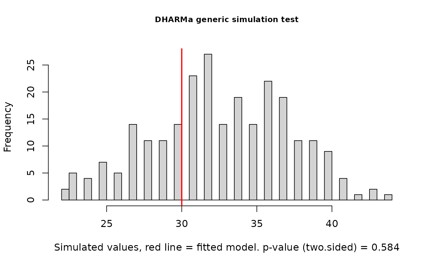 #>
#> DHARMa generic simulation test
#>
#> data: simulationOutput
#> ratioObsSim = 0.91486, p-value = 0.584
#> alternative hypothesis: two.sided
#>
testGeneric(simulationOutput, summary = countOnes, alternative = "less") # 1-deficit
#>
#> DHARMa generic simulation test
#>
#> data: simulationOutput
#> ratioObsSim = 0.91486, p-value = 0.584
#> alternative hypothesis: two.sided
#>
testGeneric(simulationOutput, summary = countOnes, alternative = "less") # 1-deficit
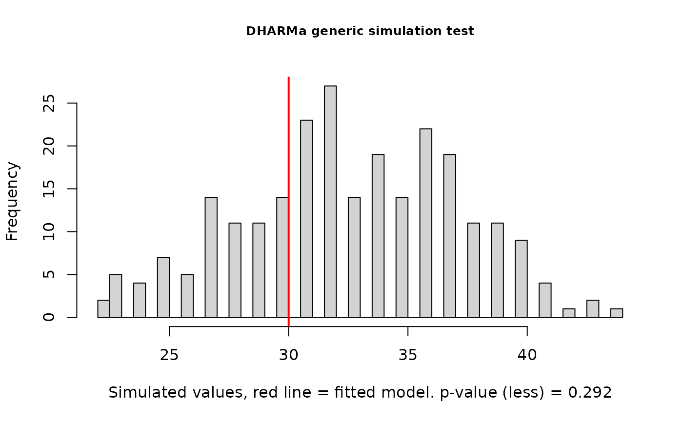 #>
#> DHARMa generic simulation test
#>
#> data: simulationOutput
#> ratioObsSim = 0.91486, p-value = 0.292
#> alternative hypothesis: less
#>
means <- function(x) mean(x) # testing if mean prediction fits
testGeneric(simulationOutput, summary = means)
#>
#> DHARMa generic simulation test
#>
#> data: simulationOutput
#> ratioObsSim = 0.91486, p-value = 0.292
#> alternative hypothesis: less
#>
means <- function(x) mean(x) # testing if mean prediction fits
testGeneric(simulationOutput, summary = means)
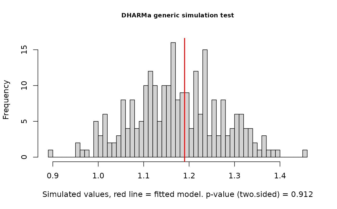 #>
#> DHARMa generic simulation test
#>
#> data: simulationOutput
#> ratioObsSim = 1.0104, p-value = 0.912
#> alternative hypothesis: two.sided
#>
spread <- function(x) sd(x) # testing if mean sd fits
testGeneric(simulationOutput, summary = spread)
#>
#> DHARMa generic simulation test
#>
#> data: simulationOutput
#> ratioObsSim = 1.0104, p-value = 0.912
#> alternative hypothesis: two.sided
#>
spread <- function(x) sd(x) # testing if mean sd fits
testGeneric(simulationOutput, summary = spread)
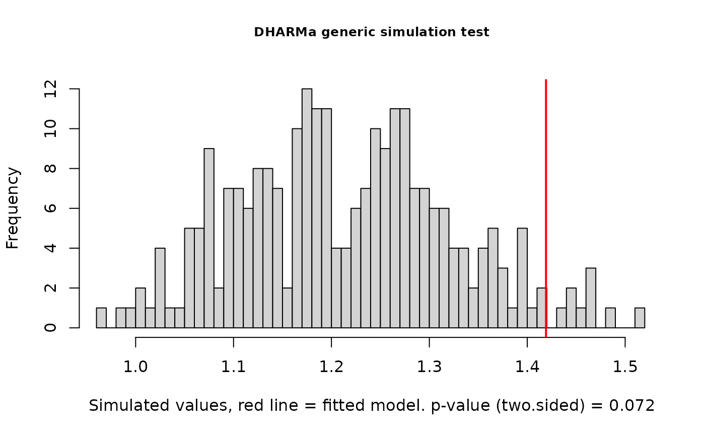 #>
#> DHARMa generic simulation test
#>
#> data: simulationOutput
#> ratioObsSim = 1.1685, p-value = 0.072
#> alternative hypothesis: two.sided
#>
#>
#> DHARMa generic simulation test
#>
#> data: simulationOutput
#> ratioObsSim = 1.1685, p-value = 0.072
#> alternative hypothesis: two.sided
#>